 |
In order to focus an image, Ekos needs to establish a numerical method for gauging how good your focus is. It's easy when you look at an image and can see it as unfocused, as the human eye is very good at detecting that, but how can Ekos possibly know that?
The most tried and tested method is Half-Flux-Radius (HFR), which is a measure of the width in pixels counting from the center of the star until the accumulated intensity is half of the total flux of the star. As you move closer to the point of optimum focus, so the HFR gets smaller, reaching a minimum at the point of focus before increasing as you start to move away from focus. HFR has been used on lots of different types of equipment and has proved to be stable in a wide range of circumstances.
In addition to HFR, Ekos supports other focus measures, including an adjusted HFR measure, FWHM, Number of Stars and Fourier Power. It is recommended to start with HFR and when the user has become proficient in focusing their equipment, to try the other measures.
After Ekos processes an image, it selects either a single star and starts measuring its HFR, or it selects a set of stars matching the criteria that have been set and calculates an average HFR. It can automatically select stars, or you can select a single star manually. It is recommended to allow Ekos to select a set of stars.
Ekos supports 4 different focus algorithms: Linear 1 Pass, Linear, Iterative, Polynomial. Linear 1 Pass is the recommended algorithm.
Linear 1 Pass: In the Linear 1 Pass algorithm, Ekos establishes a V-Curve and fits a curve to the data to find the focus solution. It then moves to the calculated minimum. Key features include:
The algorithm compensates for focuser backlash.
The algorithm is fast, taking 1 pass to identify optimum focus.
The algorithm uses more sophisticated curve fitting to pinpoint the optimum focus position.
The algorithm is highly configurable with user control over many parameters like step size, number of steps and how to deal with outliers in the datapoints.
Providing the focuser behaves in a repeatable way, i.e. when commanded to go to position X, it always goes to the same position, then this algorithm will be the best to use.
Linear: In the Linear algorithm, Ekos steps outward from its starting point then moves inward taking regular datapoints through the point of optimum focus and then further inward, to draw a V-Curve. It then fits a quadratic curve to the datapoints and calculates the point of optimum focus. It then moves out again past the point of optimum focus, halves the stepsize and moves in again for a second pass. It looks to follow the curve from the first pass and find the minimum HFR. Due to randomness in the HFR measurements it uses the % tolerance to help decide when it has found a solution. Key features include:
The algorithm compensates for focuser backlash.
The algorithm is slow, taking 2 passes to identify optimum focus.
The algorithm uses curve fitting to pinpoint the optimum focus position in pass 1, but then uses % Tolerance to try to stop as close as possible to this HFR on pass 2.
The algorithm is highly configurable with user control over many parameters like step size and number of steps.
If the focuser behaves in an inconsistent way, i.e. when commanded to go to position X, there is variability in the position it goes to, then this algorithm will be the best to use as it has some built in tolerance for this variability.
Iterative: In the Iterative algorithm, Ekos operates iteratively by moving in discrete steps, decided initially by the user-configurable step size and later by the slope of the V-Curve, to get closer to the optimal focus position where it then changes gears and performs smaller, finer moves to reach the optimal focus. The focus process stops when the measured HFR is within the configurable tolerance of the minimum recorded HFR in the process. In other words, whenever the process starts searching for a solution within a narrowly limited range, it checks if the current HFR is within % difference compared to the minimum HFR recorded, and if this condition is met then the Autofocus process is considered successful. The default value is set to 1% and is sufficient for most situations. The Step options specify the number of initial ticks the focuser has to move. If the image is severely out of focus, we set the step size high (i.e. greater than 250). On the other hand, if the focus is close to optimal focus, we set the step size to a more reasonable range (less than 50). It takes trial and error to find the best starting tick, but Ekos only uses that for the first focus motion, as all subsequent motions depend on the V-Curve slope calculations. Key features include:
The algorithm relies on the focuser having well controlled backlash.
The algorithm can be fast using a minimum number of steps.
The algorithm works on a "good enough" paradigm whereby it stops when the HFR is within % Tolerance of the perceived minimum.
Polynomial: In the Polynomial algorithm, the process starts off in Iterative mode, but once we cross to the other side of the V-Curve (once HFR values start increasing again after decreasing for a while), then Ekos performs quadratic curve fitting to find a solution that predicts the minimum possible HFR position. Key features include:
The algorithm relies on the focuser having well controlled backlash.
The algorithm can be fast using a minimum number of steps.
The algorithm uses curve fitting to pinpoint the optimum focus position.
 |
The Optical Train group displays the currently selected Optical Train. By default this will be the primary imaging train, but other trains can be selected. The group consists of:
: The Optical Train currently in use by the Focus tab. Hover the mouse over this field for a more detailed description of the selected train.
: Brings up the Optical Train dialog to view and potentially change the optical trains.
Focus parameters are saved per Optical Train automatically and so multiple trains can be setup to manage different configurations with different parameters.
When a new Optical Train is created, Focus will attempt to default parameters from other, similar Optical Trains. The attributes that must match for this are the Focuser and the scope type. If this is the first train for the selected Focuser and scope type then default parameters are created.
It is recommended to use the Focus Advisor tool on new Optical Trains to set parameters appropriately.
 |
All INDI-compatible focusers are supported. It is recommended to use absolute focusers for the best results since their absolute position is known on power up. In INDI, the focuser zero position is when the drawtube is fully retracted. When focusing outwards, the focuser position increases, while it decreases when focusing inwards. The following focuser types are supported:
Absolute: Absolute Position Focusers such as RoboFocus, MoonLite, ASI ZWO
Relative: Relative Position Focusers.
Time Based: Time based focusers with no position feedback that adjust focus position by moving for a certain amount of time.
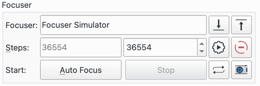
The field contains the focuser in the attached Optical Train.
For absolute and relative focusers, the step size is in units of ticks and for simple, or time based, focusers, the step size is in milliseconds. The and buttons can then be used to move the focuser by the number of ticks defined in the field in the Mechanics tab.
The Steps fields has 2 parts:
Left Hand Steps: Current focuser position. This is output only and is updated as the focuser moves to reflect the current position.
Right Hand Steps: This is input and allows the user to enter a desired position. When the button is pressed, the focuser is moved from its current position to the position indicated in this field.
On startup, the Left Hand Steps will show the current focuser position. The Right Hand Steps field is defaulted from the Optical Train saved settings. This is useful, for example, if you have several Optical Trains that use the same focuser but solve at different positions. In this case, the Right Hand Steps will contain the last persisted value for this field for the selected Optical Train. So, after swapping equipment and selecting the Optical Train, if the user presses the button then the focuser will be moved to a good place to start focusing from.
The button moves the focuser to the position in the righthand Steps field.
The button stops the in-progress focuser motion.
The button starts an Autofocus run. The button is used to stop the run.
The button will take a frame based on the current settings in the Camera & Filter Wheel Group. The button will start repeatedly capturing frames until the button is pressed.
Some of the focus algorithms will attempt to cope with being started away from the point of optimum focus, but for predictable results, it is best to start from a position of being approximately in focus. For first time setup, can be used along with the and buttons to adjust the focus position to roughly minimize the HFR of the stars in the captured images. When Framing is used in this way, the V-Curve graph changes to show a time series of frames and their associated HFRs. This makes the framing process much easier to perform.
If you are completely new to astronomy, it is always a good idea to get familiar with your equipment in daylight. This includes getting the approximate focus position on a distant object. This will provide a good starting position for focusing on stars when nighttime comes.
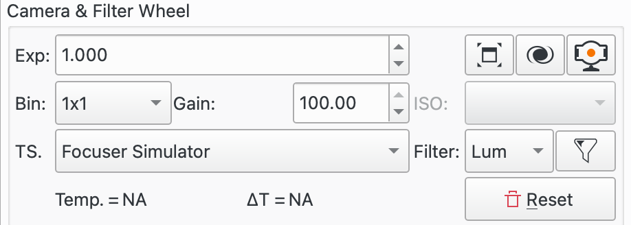 |
This section of parameters deals with the Camera and Filter settings to use when focusing.
The top row of controls allows CCD parameters to be set.
Exp: The exposure time in seconds.
The button pops the window displaying the focus frame out to a separate window. Pressing it again returns it within the focus window.
The button pops-up a separate FITS Viewer window to display the focus frame, in addition to the focus frame displayed within the focus window.
The button brings up the associated popup.
The next row of controls allows Camera parameters to be set. Choose a value from the binning dropdown and then set either the camera gain or ISO.
Binning: Increasing the binning will change the image scale as well as resulting in brighter pixels. It is generally only worth binning above 1x1 if your image scale is oversampled where the increase in image scale does not lead to a loss of resolution. If you wish to increase star brightness try increasing the exposure and / or gain. If you are unsure bin 1x1.
Gain: Set the Gain for the Camera being used to focus. The value needs to be high enough to give a clear star pattern but not so high as to create too much noise to interfere with the focus operation. Some experimentation will be required to find an optimum value. If you are unsure where to start try unity gain for your camera and adjust from there.
ISO: Set the ISO for the Camera being used to focus. Some experimentation will be required to find an optimum value.
The third row of controls deals with the Temperature Source and Filter, if there is one:
TS: Select the temperature source from the dropdown. Underneath are displayed the current temperature from the selected temperature source and the change in temperature between when the last successful Autofocus run completed and the current temperature. It is common practice to redo focus after significant temperature changes that alter the telescope's focus point.
Filter: Select the filter to use.
To start focusing it will probably be easier to select the filter that allows the most light through, for example the Lum filter. Click the filter icon
 to launch the Filter Settings
popup. This allows a number of parameters to be set per filter to be used during
an Autofocus run.
to launch the Filter Settings
popup. This allows a number of parameters to be set per filter to be used during
an Autofocus run.button will reset the focusing subframe to full frame.
 |
This section describes the focus tools that are currently available.
The button starts an Aberration Inspector run. The button can be used to stop the run.
The button launches the Critical Focus Zone tool.
The button launches the Focus Advisor tool.
The Force AF checkbox can be used when a sequence is active either in Capture or the Scheduler. When checked, an Autofocus will be triggered at the completion of the currently active subframe.
 |
Parameters to configure Focus are accessed by pressing the button. This launches the Options dialog with three panes:
The parameters are stored for each Optical Train. This allows different configurations to be stored for different equipment. Parameters are stored when they are changed, so on startup the last used configuration for the selected Optical Train is loaded.
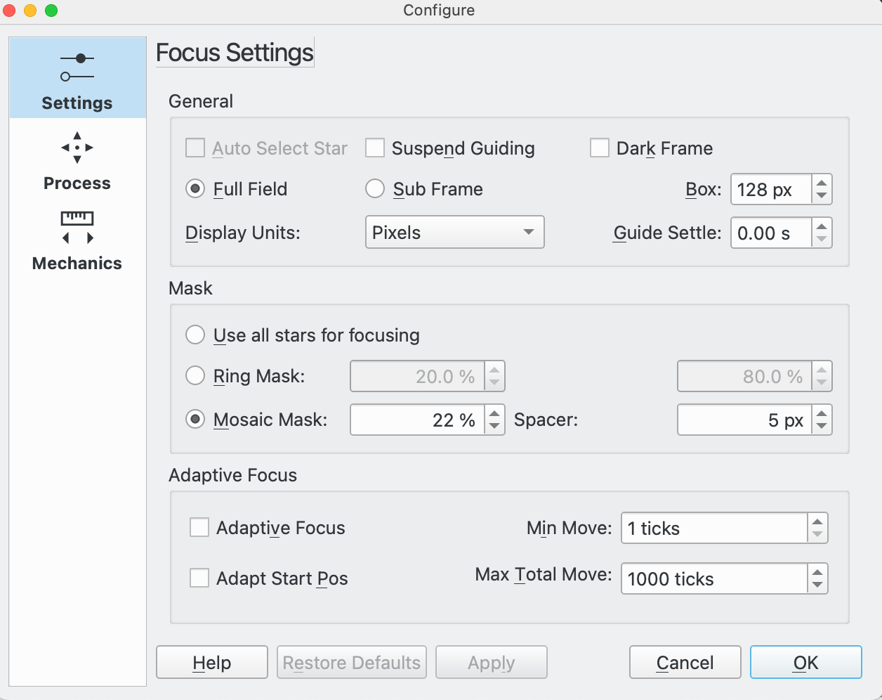 |
General section parameters:
Auto Select Star: This setting is only relevant if Sub Frame is selected. In this case if Auto Select Star is selected then Ekos will select the star to use for focus; otherwise the user will have to manually select the star using FitsViewer.
Suspend Guiding: Set this option to suspend guiding during an Autofocus run. The purpose of this is to prevent guiding from having problems with defocused stars during the focus process where, for example, the guide scope is attached to the main telescope using an OAG.
Dark Frame: Check this option to perform dark-frame subtraction. This option can be useful in noisy images, where a pretaken dark is subtracted from the focus image before further processing.
If hot pixels are causing problems with focus, select Dark Frames and either setup a regular Master Dark frame or a Defect Map.
Dark frames are used by Focus, Alignment and Guiding. See the Dark Library feature within the Capture Module for more details on how to setup Dark Frames.
Full Field: Select to use the full field of the camera. In this mode, focus will automatically select multiple stars for use in an Autofocus run. The alternative to this is Sub Frame.
Sub Frame: Select to use a single star for the Autofocus process. The alternative to this is Full Field where multiple stars will be used by Autofocus. Depending on the setting of Auto Select Star either the user or Ekos will select the star.
Box: Sets the box size used to enclose the focus star when using Sub Frame. Increase if you have very large stars. For Bahtinov focus the box size can be increased even more to better enclose the Bahtinov diffraction pattern.
Display Units: Select the units for display on the Autofocus V-Curve when HFR or FWHM is selected. Pixels and Arc Seconds are supported.
Guide Settle: This option is used in conjunction with Suspend Guiding. It allows any vibrations in the optical train to settle by waiting this many seconds after the Autofocus process has completed, before restarting guiding.
Mask Section Parameters:
These controls relate to Masking Options to be used when in Full Field mode. The effect of Masking Options can be seen in the FITS Viewer.
Use all stars for focusing: Select this option if all stars of the field should be considered for focusing.
Ring Mask: This option provides two input fields that together define a doughnut over the FOV of the camera. Stars falling outside of the doughnut are discounted from processing. Setting an inner value above 0% causes stars in the centre of the FOV to be discarded. This could be useful to avoid using stars in the target of the image (for example a galaxy) for focusing purposes. Setting an outer value below 100% causes stars in the edges of the FOV to be discarded during focusing. This could be useful if you do not have a flat field out to the edges of your FOV.
Mosaic Mask: A 3x3 mosaic is composed with tiles from the image center, its corners and from the edges. This option is useful if you want to inspect the optics performance - you might know this from the PixInsight Aberration Inspector script. The tile size can be configured in percent of the frame width, with the spacer value specifying the space between the tiles.
There are four use-cases for the Mosaic Mask:
Checking focus in all parts of the sensor: The mask allows an easy visual inspection and comparisons of stars in the center, corners and edges of the sensor. This is especially useful for optics that show aberration if the focus is not 100% met.
Correcting image tilt: especially large sensors are very sensitive to incorrect distance and tilting of the sensor. In such cases, the image shows aberration, especially in the image corners. If all corners show the same effect, the distance needs to be corrected. If the aberrations in the corners differ, this is typically the result of a tilted sensor.
Collimating Newtonians: inspecting frames in a defocused state is typically used for collimating Newtonians. See, for example, Tommy Nawratil's The Photonewton Collimation Primer for more details.
Running the Aberration Inspector tool.
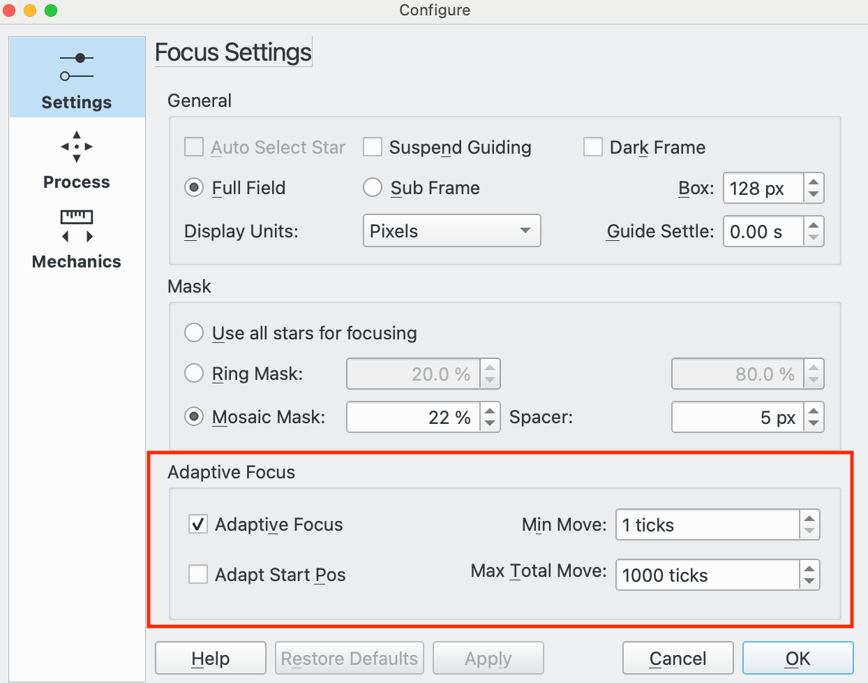
Adaptive Focus Parameters:
The next set of controls relate to Adaptive Focus. The idea here is to keep the telescope focused by adapting the focuser position based on changes in environmental conditions without having to perform a full Autofocus run. See the Adaptive Focus section for more details.
For example, as temperature changes during an imaging session so the focus point will change. By sampling the temperature between subframes it is possible to firstly calculate the change in temperature and then to convert this to a number of ticks of focuser movement to apply between subframes.
In order to use Adaptive Focus it is necessary
to setup some data for your system. In particular you need to tell Ekos how many ticks (and
in which direction) to move the focuser when the environmental conditions change. This is
covered in the Filter Settings popup. The
popup is launched by clicking the filter icon .
The following controls are available:
Adaptive Focus: Select this option to activate Adaptive Focus.
Min Move: The minimum Adaptive Focus movement allowed.
Adapt Start Pos: Check to allow Adaptive Focus to calculate the start position for an Autofocus run. The starting position is the last good solve position for the selected filter, adapted for environmental changes.
For example, if the current focuser position is 1000, temperature = 4C, and if the Red filter is selected (last good focus position for Red is 990 @ 5C and Ekos is configured to move +3 Ticks / °C). Then, if Adapt Start Pos is off, Autofocus will start at 1000. If Adapt Start Pos is on, Autofocus will start at 990 + (5 - 4) * 3 = 993.
This feature is useful to ensure that Autofocus starts from close to the focus point which will mean a more symmetric V-curve. It is particularly useful when changing between filters which have large differences in focus points.
It is possible to use this feature on its own without Adaptive Focus. Just set the checkbox and leave the ticks per degree C set to zero. This way the Autofocus start position will be filter dependent and will start each Autofocus run at the focus point of the last successful Autofocus run for that filter.
Max Total Move: The maximum total focuser movement that Adaptive Focus is allowed in the observing session. The purpose of this is as a "dead man's handle" on Adaptive Focus in case it runs away. For example, if the temperature source fails and returns bad temperature readings whilst the equipment is unattended, this could result in Adaptive Focus attempting to make large focuser movements.
If the Max Total Move is reached then Adaptive Focus is unchecked until manually re-checked by the user.
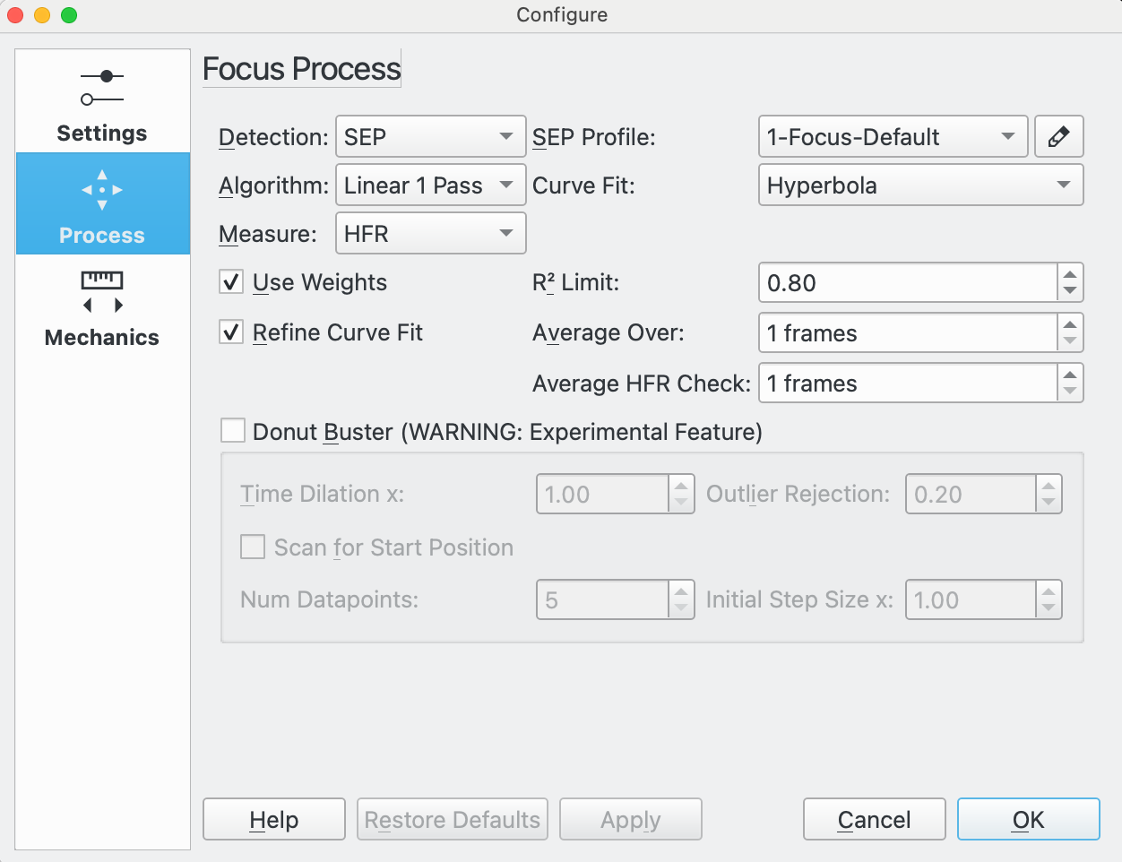 |
Focus Process Parameters:
Detection: Select star detection algorithm. Each algorithm has its strengths and weaknesses. It is recommended to use SEP, unless you have a specialized use. The following are available:
SEP: Source Extraction and Photometry built in library. This is the default value.
Centroid: An extraction method based on estimating star mass around signal peaks.
Gradient: A single source extraction model based on the Sobel filter.
Threshold: A single source detection algorithm based on pixel values.
Bahtinov: This detection method can be used when using a Bahtinov mask for focusing. First take an image, then select the star to focus on. A new image will be taken and the diffraction pattern will be analysed. Three lines will be displayed on the diffraction pattern showing how well the pattern is recognized and how good the image is in focus. When the pattern is not well recognized, the Num. of rows parameter can be adjusted to improve recognition. The line with the circles at each end is a magnified indicator for the focus. The shorter the line, the better the image is in focus.
SEP Profile: If the star detection algorithm is set to SEP, then choose a parameter profile to use with the algorithm. The following are recommended:
1-Focus-Default: for scopes that do not have a central obstruction such as a refractor.
1-Focus-Default-Donut: for scopes that have a central obstruction such as a Newtonian, SCT, RASA, Ritchey-Cretien, etc.
Algorithm: Select the Autofocus process algorithm:
Linear 1 Pass: This is the recommended algorithm. In this algorithm, Ekos establishes a V-Curve and fits a curve to the data to find the focus solution. It then moves to the calculated solution.
This algorithm supports the older style Quadratic curve type as well as the newer Levenberg-Marquardt Solver for Hyperbolic and Parabolic curves. It will also weight the datapoints in the curve fitting process if Use Weights is checked and run a refinement process if Refine Curve Fit is selected.
Linear: This algorithm builds a V-Curve with approximately Out step Multiple steps on each side of the minimum. Having built the V-Curve it then fits a quadratic equation to the curve (parabolic shape) and uses this to calculate the focuser position giving the minimum HFR. Having identified the minimum it then performs a 2nd pass halving the step size, recreating the curve from the 1st pass. It attempts to stop within Tolerance of the minimum HFR calculated during the 1st pass.
Iterative: Moves focuser by discreet steps initially decided by the step size. Once a curve slope is calculated, further step sizes are calculated to reach an optimal solution. The algorithm stops when the measured HFR is within Tolerance of the minimum HFR recorded in the procedure.
Polynomial: Starts with the iterative method. Upon crossing to the other side of the V-Curve, polynomial fitting coefficients along with possible minimum solution are calculated. This algorithm can be faster than a purely iterative approach given a good data set.
Curve Fit: The type of curve to fit to the datapoints.
Hyperbola: Fits a Hyperbola using a non-linear least squares algorithm supplied by GSL (GNU Science Library). See Levenberg-Marquardt Solver for more details.
This is the recommended option.
Parabola: Fits a Parabola using a non-linear least squares algorithm supplied by GSL (GNU Science Library). See Levenberg-Marquardt Solver for more details.
Quadratic: Uses a quadratic equation using a linear style least squares algorithm supplied by GSL (GNU Science Library). This is, in effect, a parabolic curve.
It is no longer recommended to use this curve.
Measure: Select Measure to use in the focus process. The following are available:
HFR: Half Flux Radius (HFR) is the recommended measure. When a star is detected, Ekos will calculate the HFR for the star. This is the radius of an imaginary circle, centered on the star center, that encloses half the star's total flux.
The point of best focus corresponds to the minimum HFR.
HFR Adj: This feature uses a brightness adjusted HFR calculation to take account of the fact that the HFR for brighter stars is larger than for smaller stars.
The algorithm adjusts the value of the measured HFR, usually upwards, so the HFRs obtained by the HFR Adj method will be higher than the measured HFR values. This does not mean that you are getting worse results by using HFR Adj, simply that the measure is different.
When using this Measure it is usual to get smaller error bars on the datapoints when Use Weights is selected.
The point of best focus corresponds to the minimum adjusted HFR.
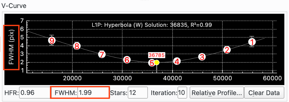
FWHM: This feature fits a Gaussian surface to each star and uses that to calculate the Full Width Half Maximum (FWHM) of the star. The FWHM is the width of an circle (or ellipse) centered on the star center reaching the edge of the star at half its maximum intensity.
The point of best focus corresponds to the minimum FWHM.
Expect the FWHM to be approximately twice the HFR of a star.
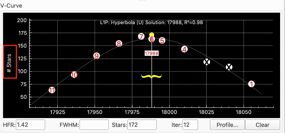
# Stars: This feature calculates the number of stars in the image and uses this number as the focus measure. The idea is that as you move nearer focus so more stars become detectable.
The advantage of this Measure is that it is very simple and does not require algorithms to calculate HFRs or FWHMs.
The point of best focus corresponds to a maximum number of stars.
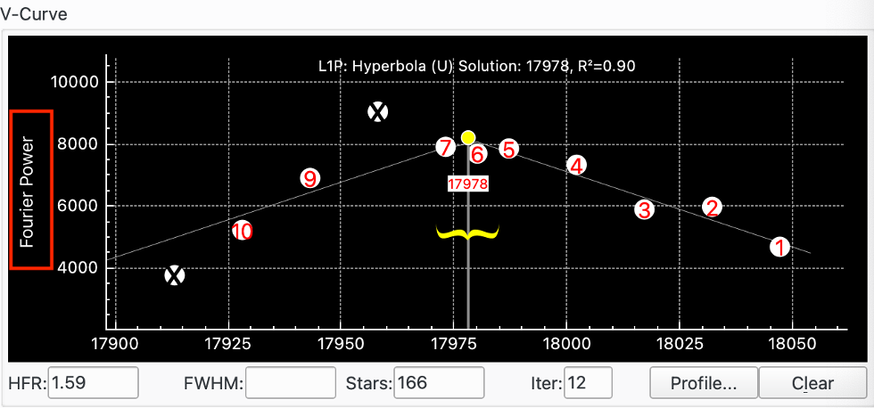
Fourier: Fourier takes a Fourier transform of the image and calculates the image power in frequency space. The assumption is that for an astronomical image of stars and background, the stars will be gaussians. Under a Fourier transform, a gaussian transforms to another gaussian; but wider stars transform to narrower gaussians in frequency space, and vice-versa. So, at focus, summing up the contents in frequency space, which is in effect a measure of power, will be a maximum.
This follows the main idea suggested by Tan and Schulz in their paper: A Fourier method for the determination of focus for telescopes with stars. Please note that this paper makes other processing suggestions beyond the idea of using Fourier Transforms that are not included within Ekos
This is a relatively new method in the Astro Community, and does not require star detection. Tan and Schulz report good results with both amateur and professional telescopes.
PSF: If Measure is set to FWHM, then the PSF widget can be selected for use in fitting a surface to the star. At present just Gaussian is supported.
Use Weights: This is only available with the Linear 1 Pass focus algorithm and Curve Fits of Hyperbola and Parabola. It requires Full Field to be selected. The option calculates the standard deviation of star Measure and uses the square of this (mathematically the variance) as a weighting in the curve fitting process. The advantage of this is that datapoints with less reliable data and therefore larger HFR standard deviations will be given less weight than more reliable datapoints. If this option is unchecked, and for all other curve fitting where the option is not allowed, all datapoints are given equal weight in the curve fitting process.
The standard deviation is drawn on the V-Curve for each datapoint as an error bar.
It is recommended to check this option.
See the Levenberg-Marquardt Solver for more details.
R² Limit: This is only available with the Linear 1 Pass focus algorithm and Curve Fits of Hyperbola and Parabola. As part of the Linear 1 Pass algorithm, the degree to which the curve fits the datapoints, or Coefficient of Determination, R², is calculated. This option allows a minimum acceptable value of R² to be defined that is compared to the value obtained from the curve fitting process. If the minimum value has not been achieved then Autofocus will rerun. Only one rerun will be performed and even if the minimum R² has not been met the second time, the Autofocus run will still be deemed successful.
Experiment to find an appropriate value but a good starting point would be 0.8 or 0.9
Refine Curve Fit: This option is only available with the Linear 1 Pass focus algorithm and Curve Fits of Hyperbola and Parabola. If this option is checked then at the end of the sweep of datapoints, Ekos fits a curve and measures the R². It then applies Peirce's Criterion based on Gould's methodology for outlier identification. See Peirce's Criterion for details incl Peirce's original paper and Gould's paper which are both referenced in the notes. If Peirce's Criterion detects 1 or more outliers then another curve fit is attempted with the outliers removed. Again the R² is calculated and compared with the original curve fit R². If the R² is better, then the latest run is used, if not, the original curve fit (with the outliers included) is used.
Outliers are clearly marked on the V-Curve with an X through the datapoint.
It is recommended to check this option.
Average over: Number of frames to capture at each datapoint. It is usually sensible to start with 1 but increasing this will result in an averaging process for the star Measure selected.
Average HFR check: Similar idea to Average Over but in this case it is the HFR Check datapoint that is averaged over the selected number of frames. In addition, if the Algorithm is Linear 1 Pass then the last datapoint of an Autofocus run, which is the in-focus datapoint, is also averaged over this number of frames. Set a value of 1 to start. This can be increased if there are issues with HFR Check Autofocus runs being triggered by outlying datapoints when the HFR Check runs.
Donut Buster: This is an experimental feature and should be used with caution. The intention of Donut Buster is to improve focusing for telescopes with central obstructions that create donut shaped stars when defocused, e.g. Newtonians, SCTs, RASAs, Ritchey-Cretiens, etc.
Donut Buster is only available for Linear 1 Pass, walks of Fixed and CFZ Shuffle, curves fits of Hyperbola and Parabola, and focus measures of: HFR, HFR Adj and FWHM.
When Donut Buster is checked, intermittent curve fitting is suspended and is only activated at the end of the focus sweep. This allows donut buster to better process edge datapoints that may be affected by donuts.
The following sub-options are available within Donut Buster:
Time Dilation x: This feature scales the exposure time during Autofocus from the value entered in the Exposure field for the furthest datapoints from focus. Datapoints near focus are taken with an unscaled exposure. For example, if Focus is setup with an Exposure of 2s and Time Dilation x is set to 4, then when Autofocus moves out to take its first datapoint, an exposure of 2s * 4 = 8s is used. On each successive datapoint the exposure is reduced down to 2s around the point of optimum focus. As the focuser moves through focus, so the exposure is scaled upwards to 8s for the last datapoint.
The purpose of this feature is to increase the brightness of out of focus datapoints which will be dimmer than in-focus datapoints and therefore harder for star detection to resolve from the background noise.
Outlier Rejection: This is a factor to scale the aggressiveness of the outlier rejection algorithm when Refine Curve Fit is checked. The higher the value the more outliers will be excluded from the curve fitting process. The default value is 0.2.
Scan for Start Position: Check this option to have Focus scan around the current focuser position to find an approximate optimum focus position. The purpose of this is to ensure that Autofocus starts near to the focus position. The following sub-options are available:
Num Datapoints: The number of datapoints to use in each scan. 5 is a good place to start.
Initial Step size x: A multiplicative factor to apply to the Initial Step size for use in the Scan for Start Position. Default is 1.0.
If Detection is set to Threshold then the following additional field is available:
Threshold: This contains a percentage value used for star detection using the Threshold detection algorithm. Increase to restrict the centroid to bright cores. Decrease to enclose fuzzy stars.
If Detection is set to Bahtinov then the following additional widgets are available:
Num. of rows: The number of lines displayed on screen when using a Bahtinov mask.
Sigma: The sigma of the gaussian blur applied to the image before applying Bahtinov edge detection.
Kernel Size: The kernel size of the gaussian blur applied to the image before applying Bahtinov edge detection.
If Algorithm is set to Linear or Iterative then the following additional widget is available:
Tolerance: The tolerance percentage value is used to help decide when the Autofocus process stops. During the Autofocus process, HFR values are recorded, and once the focuser is close to an optimal position, it starts measuring HFRs against the minimum recorded HFR in the session and stops whenever a measured HFR value is within % difference of the minimum recorded HFR. Decrease the value to narrow the optimal focus point solution radius. Increase to expand solution radius.
Warning
Setting the Tolerance value too low might result in a repetitive loop and would most likely result in a failed Autofocus process.
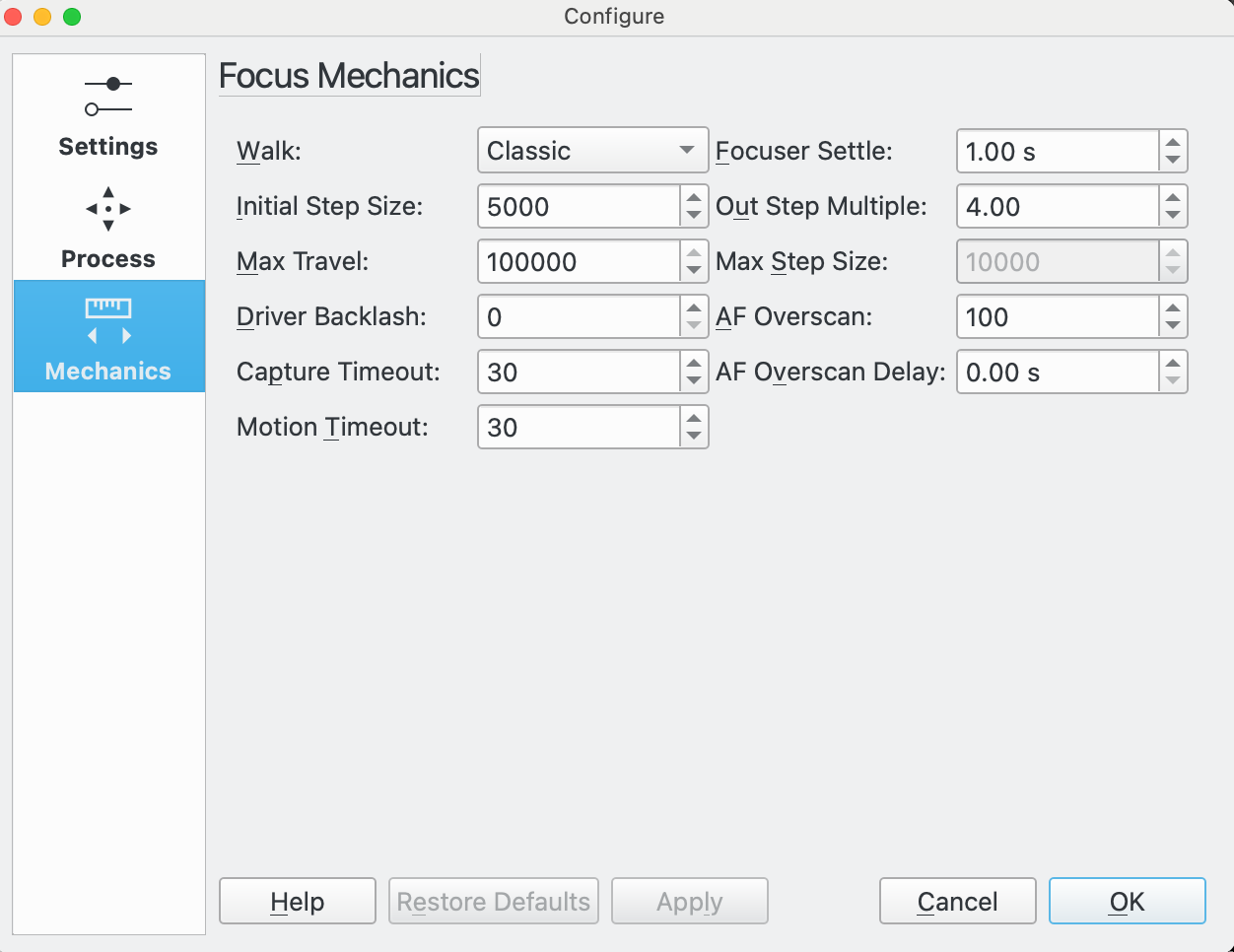 |
Focus Mechanics Parameters:
Walk: This specifies the way Autofocus will "walk" inwards through its sweep to produce the V-Curve from which the focus solution will be calculated.
The following are available:
Classic: This is the recommended setting. The inward sweep follows a series of steps of equal size (Initial Step Size). The algorithm includes logic to determine when to stop that makes the exact number of steps unpredictable but it will be about 2 * (Out Step Multiple) + 1.
This Walk is tolerant of curve fitting failures in the last step where it will take a further step and try again to solve. It is also somewhat tolerant of not being started near to focus so is a good choice for the initial Autofocus run.
Because of the "tolerance" of this Walk to less than perfect setup it is a conservative option to chose, but comes at the expense of extra steps and therefore extra time in the Autofocus process.
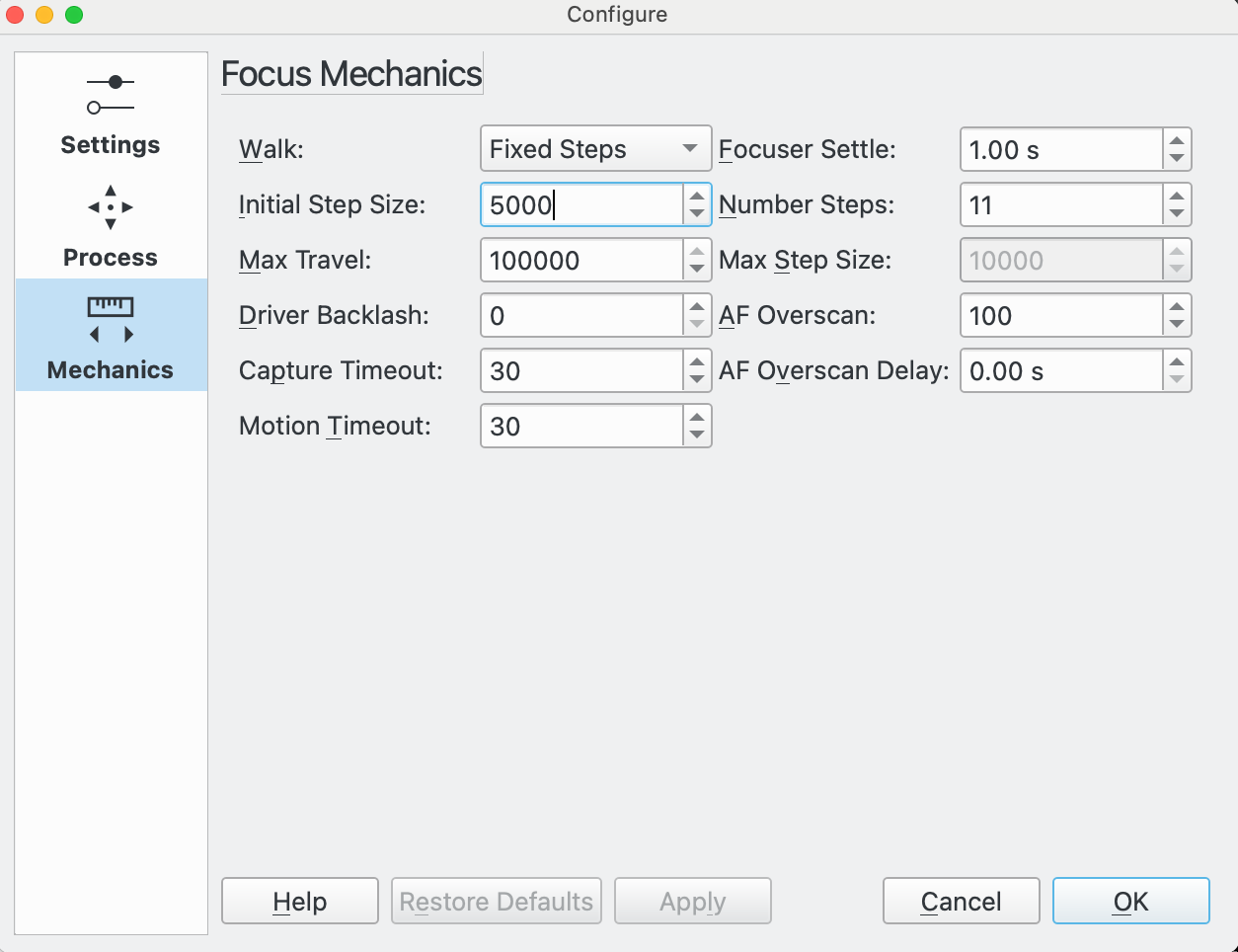
Fixed Steps: This feature is available in the Linear 1 Pass Algorithm. It is quite similar to Classic but Fixed Steps is used to control the total number of steps taken.
This algorithm is more predicable than Classic in that it takes a definite number of steps (so will be faster), but is less tolerant of issues curve fitting the last data point and needs to be started near to focus.
When selected, the Out Steps Multiple is replaced by Fixed Steps:
CFZ Shuffle: This feature is available in the Linear 1 Pass Algorithm. It is a variation on Fixed Steps so the comments on that Walk are applicable here as well.
The difference between CFZ Shuffle and Fixed Steps is that near the center of the sweep (which should be around the Critical Focus Zone (CFZ)) the algorithm takes steps of half the specified size.
Focuser Settle: The number of seconds to wait, after moving the focuser, before starting the next capture. The purpose is to stop any vibrations in the optical train from affecting the next frame.
Initial Step size: This sets the step size to be used by various focus algorithms. For absolute and relative focusers this is the number of ticks; for timer based focusers this is the number of milliseconds.
Out Step Multiple: Used by the Linear and Linear 1 Pass focus algorithms in the Classic walk, this parameter specifies the initial number of outward steps the focuser takes at the start of an Autofocus run.
Number Steps: Used by the Linear 1 Pass algorithm in the Fixed Steps and CFZ Shuffle walks, this parameter specifies the total number of steps the focuser takes to create the V-Curve in an Autofocus run.
Max Travel: Puts bounds on the amount of travel from the current focuser position that is permitted by the Autofocus algorithms. The purpose is to protect the focuser from travelling too far and potentially damaging itself. On the other hand, the value needs to be big enough to allow sufficient focuser motion to permit the auto focus runs to complete.
Max Step Size: Used by the Iterative algorithm to limit the maximum step size that can be used.
Driver Backlash: See the section on Backlash.
There are 2 schemes that can be used:
Set Driver Backlash to 0 to switch it off and deal with Backlash elsewhere.
Set Driver Backlash > 0 to use Driver Backlash to manage Backlash in the device driver. Note that this field is only editable if the device driver supports Backlash.
This is the same data field that is displayed in the Indi Control Panel for the focuser device. It can be set in either place.
AF Overscan: See the section on Backlash.
There are 2 schemes that can be used:
Set AF Overscan to 0 to switch it off and deal with Backlash elsewhere.
Set AF Overscan > 0 to have the Focus module manage Backlash.
AF Overscan Delay: Delay between the completion of the outward move of an Overscan, and the inward move. Generally most focusers work well with no delay.
Capture Timeout: The amount of time in seconds to wait for a captured image to be received before declaring a timeout. This should only be triggered if there are problems with the camera during the Focus process so set this to a high enough value that it will not occur during normal operation.
Motion Timeout: The amount of time in seconds to wait for the focuser to move to the requested position before declaring a timeout. This should only be triggered if there are problems with the focuser during the Focus process so set this to a high enough value that it will not occur during normal operation.
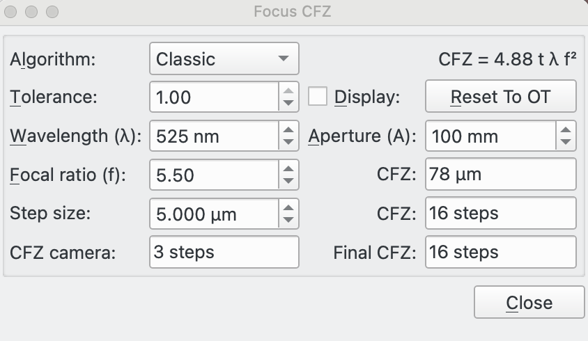 |
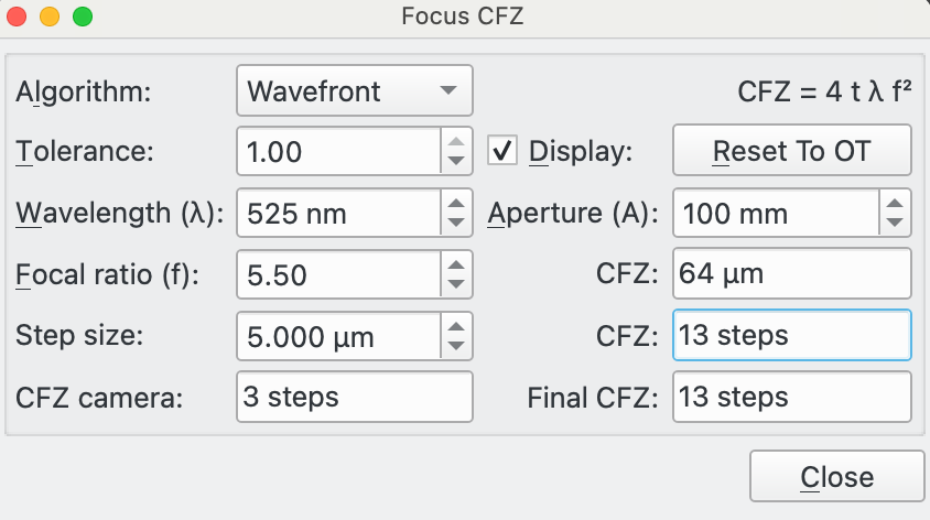
Focus CFZ Parameters:
Algorithm: This specifies the Critical Focus Zone (CFZ) algorithm. The purpose of this is to calculate the CFZ for the equipment attached in the Optical Train. It is not necessary to use this functionality in order to successfully focus, but it provides useful information if correctly configured.
It requires some knowledge to configure it correctly. There is plenty of information available on the internet.
The idea of the CFZ dialog is that it starts with data from the Optical Train used in the Focus tab and uses that to calculate the CFZ. The user can adjust parameters to do "what-if" scenarios to see how it affects the CFZ. Clicking the Reset to OT button resets any adjusted parameters to the Optical Train values.
If the Display box is checked then the CFZ is drawn on the V-Curve after Autofocus successfully completes.
It is necessary to specify the Step Size parameter which specifies in microns how far one tick moves the focal plane. For refractors there is usually a 1-to-1 relationship between moving the focuser which moves the telescope draw-tube mechanism and the focal plane movement. For other types of telescope the relationship is likely to be more complex. Refer to details of your telescope / manufacturer for this information.
The following algorithms are available:
Classic: This is the recommended setting. The equation used is displayed in the top right of the dialog and is the equation most commonly seen on the internet. The equation comes from a linear optics treatment using the Airy Disc and is acknowledged to have limitations. For this reason it includes a "tolerance" factor that can be adjusted by the user. For example, in the often quoted “In Perfect Focus” article by Don Goldman and Barry Megdal in Sky & Telescope 2010 they suggest setting t=1/3.
Wavefront: The equation used is displayed in the top right of the dialog. The equation comes from a wavefront approach to the CFZ. Again, it has limitations and again, for this reason it includes a "tolerance" factor that can be adjusted by the user.
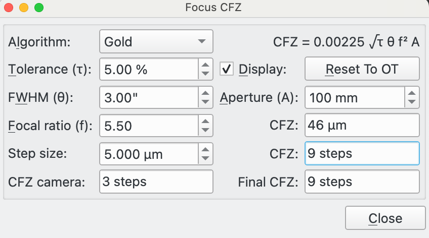
Gold: This method is based on work done by Gold Astro and presented here.
Tolerance: This is used by Classic and Wavefront algorithms and is a scaling factor between 0 and 1.
For the Classic algorithm, Goldman and Megdal suggest 1/3.
For the Wavefront algorithm, some have suggested 1/3 or even 1/10.
Tolerance (τ): This is used by the Gold algorithm and is a focus tolerance as a percentage of total seeing. The Gold website suggests 3-5% for a good focuser or 1-2% for a top quality focuser. See the Gold Astro website for more details.
Display: Check this box to display the calculated CFZ on the V-Curve after a successful Autofocus run. It is displayed as a yellow moustache.
Reset to OT: Press this button to reset any parameters to values defaulted from the currently connected Optical Train.
Wavelength (λ): This is the light wavelength to use. It is defaulted from the currently used filter. Remember to set this up in Filter Settings for your filters.
Aperture (A): This is the aperture of the telescope in mm. It is defaulted from the currently connected Optical Train.
Focal Ratio (f): This is the focal ratio of the telescope. It is defaulted from the currently connected Optical Train.
FWHM (θ): This is used by the Gold Algorithm and is the total seeing. This is the combined contribution of the diffraction limit of your telescope and the astronomical seeing. The Gold Astro website describes how you might approximate the total once you have values for the individual contributions.
CFZ: This is calculated CFZ in microns and in ticks.
Step Size: This must be input by the user (as it cannot be calculated by Ekos). It relates how far 1 tick moves the focal plane in microns.
For a refractor this is how far the drawtube moves when the focuser is moved by 1 tick. You might be able to get this value from the specification of your focuser (how many ticks for a complete revolution of your focuser) and the thread pitch of your telescope drawtube along with any gearing involved.
Alternatively, you can measure how far the drawtube moves from end to end (be careful not to force the drawtube) with a set of calipers or a ruler. By subtracting the furthest "in" position (in ticks) from the furthest "out" position (in ticks) you have how many ticks moved the drawtube the distance you measured. From this you can calculate the distance in microns a single tick moves the drawtube.
Other types of telescope will have other ways to adjust the focal plane, for example, by moving the primary or secondary mirrors. You will need to either get the Step Size from the documentation for your equipment or work out how to measure it in a way that are consistent with that described above.
CFZ Camera: The pixel size of the camera attached via the Optical Train may have a limiting effect on the CFZ. So an equivalent CFZ for the attached camera is calculated assuming a Nyquist 2* limit.
Final CFZ: This is the larger of the CFZ calculated using the selected algorithm for the specified parameter and the CFZ Camera. It is the display value and is, in effect, the CFZ of your equipment.
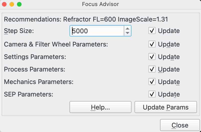 |
This is the Focus Advisor dialog. It is a feature to assist with management of focus parameters.
The purpose of Focus Advisor is to help people struggling to use the Focus module within Ekos. The Focus module is functionally rich and contains a lot of parameters that need to be set self-consistently to achieve good results. Focus Advisor is designed to help with basic parameter setup that should achieve focus. It is not designed to achieve the best possible focus for your equipment; you will have to experiment with your setup to achieve that. But Focus Advisor provides a place to start that experimentation.
So Focus Advisor is aimed towards the less experienced users.
If Focus Advisor does not appear to give good results on your setup why not start a discussion on the forum so it can be enhanced to give better results in the future. This way it will build over time to be more useful.
When you click on Focus Advisor it works out a series of parameter recommendations based on the Optical Train you are using in Focus.
At the top of the dialog it displays information about the connected Optical Train. Then it displays 6 lines relating to various sets of parameters used within Focus. Against each line is a checkbox to update the associated Focus fields with Focus Advisor's recommendations.
Focus parameters are broken into the following groupings:
Step Size: This is the suggested focus step size to use. This is a critical parameter. It can be defaulted from the Critical Focus Zone (CFZ) dialog if you know how to set that up. Alternatively, if you know a reasonable value for your equipment from other sources you can just enter that.
Camera & Filter Wheel Parameters: This sets the parameters in the CCD & Filter Wheel section of the Focus screen. By hovering the mouse over this label you can see in the tooltip what values Focus Advisor is recommending.
Settings Parameters: This sets the parameters in Focus Settings. By hovering the mouse over this label you can see in the tooltip what values Focus Advisor is recommending.
Process Parameters: This sets the parameters in Focus Process. By hovering the mouse over this label you can see in the tooltip what values Focus Advisor is recommending.
Mechanics Parameters: This sets the parameters in Focus Mechanics. By hovering the mouse over this label you can see in the tooltip what values Focus Advisor is recommending.
SEP Parameters: This sets the SEP parameter profile appropriate for the scope type attached in the selected Optical Train. By hovering the mouse over this label you can see in the tooltip what values Focus Advisor is recommending.
Help: Press this button to get help on using Focus Advisor.
Update Params: Press this button to accept the Focus Advisor recommendations and update the Focus parameters where the associated Update checkbox is checked..
 |
Click the filter icon from either Capture or Focus to open the filter settings dialog. This popup allows the user to
configure data associated with each filter, and used for various functions within the system.
Focusing with different filters can be done in one of three ways within Ekos.
Direct Autofocus: When Capture changes to this filter it is possible to automatically refocus this filter. The exposure to use for the selected filter is taken from the Exposure field. This allows, for example, narrowband filters to use a longer exposure than broadband filters during Autofocus.
Check Auto Focus to use the filter in this way.
Autofocus on Lock Filter: It is possible to specify a Lock filter to use when it is required to focus this filter. For example, if the Ha filter is used and an Autofocus run required, it is possible to run Autofocus using the Lum filter and then, when complete, adjust the focus position by an Offset value corresponding to the predetermined focus difference between the Lum and Ha filters (100 ticks in this example). This is useful when, for example, it is difficult to focus some filters directly without excessively long exposure times. Note that this locked filter approach may also be used in the Alignment Module whenever it performs a capture for astrometry.
To use a filter in this way, check Auto Focus, specify the Lock Filter to use and make sure that the Offsets for this filter and the Lock Filter are set.
Use Offsets: It is possible to use filter offsets to adjust focus when swapping between filters, without running Autofocus. This requires some setup work ahead of time but has the advantage of reducing the number of Autofocus runs and therefore reducing the time spent autofocusing.
In order to use this feature it is necessary to work out the relative focus position between all filters that you wish to use this functionality for. For example, if Lum and Red have the same focus position (they are parfocal) but Green focuses 300 ticks further out than Lum (or Red) then setup Offsets for Lum, Red and Green as 0, 0, 300 as shown above. If a sequence is created to take 10 subframes of Lum, then 10 Red, then 10 Green, then at the start, since Lum has Auto Focus checked, an Autofocus will be run on Lum and the 10 subs taken. Capture will then switch filters to Red. Since Red has Auto Focus unchecked no Autofocus will happen and Ekos will look to the Offsets between Red and Lum. In this case 0 - 0 = 0. So the focuser will not be moved and Capture will take 10 subs of Red. Then Capture will swap from Red to Green. Again, Green has Auto Focus unchecked no Autofocus will happen and Ekos will look to the Offsets between Green and Red. In this case 300 - 0 = 300. So Focus will adjust the focus position by +300 (move the focuser out by 300 ticks). Capture will then take the 10 Green subs.
To use a filter in this way, uncheck Auto Focus and make sure that the Offsets for this filter and all other filters that can precede this filter in a sequence are set.
The Offsets can either be worked out by running Autofocus with different filters and manually calculating the relative offsets and entering them into the table or by using the Build Offsets tool.
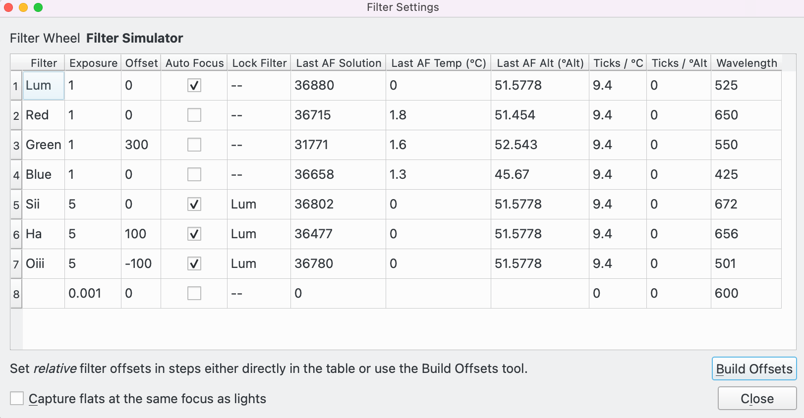
Configure settings for each filter in the table:
Filter: Filter Name.
Exposure: Set exposure time (in seconds) to be used when performing Autofocus on this filter. By default, it is set to 1 second.
Offset: Set relative offsets. Ekos will command a focus offset change if there is a difference between the current and target filter offsets. For example, given the values in the example image, if the current filter is set to Red and next filter is Green, then Ekos shall command the focuser to Focus In by +300 ticks. Relative positive focus offsets denote Focus Out while negative values denote Focus In.
Auto Focus: Check this option to perform AutoFocus whenever the filter is changed to this filter.
Lock Filter: Set which filter should be set and locked when performing autofocus for this filter. "--" indicates no Lock Filter. It is not allowed to next filters more than 1 deep, i.e. Red cannot be locked to Blue which is itself locked to Green. A filter cannot be locked to itself.
Last AF Solution: The last successful Autofocus position. Under normal operation Ekos will automatically update this field.
Last AF Temp (°C): The temperature of the Last AF Solution. Under normal operation Ekos will automatically update this field.
Last AF Alt (°Alt): The altitude of the Last AF Solution. Under normal operation Ekos will automatically update this field.
Ticks / °C: The number of ticks to move the focuser when the temperature changes by 1°C. For example, if focus moves out by 5 ticks when temperature increases by 1°C, set this field to 5. If focus moves in by 5 ticks when temperature increases by 1°C, set this field to -5.
Ticks / °Alt: The number of ticks to move the focuser when the altitude changes by 1°Alt. For example, if focus moves out by 0.5 tick when altitude increases by 1°Alt, set this field to 0.5. If focus moves in by 0.5 tick when altitude increases by 1°Alt, set this field to -0.5.
Wavelength: The center of the passband of the filter in nanometers. This is used in some Critical Focus Zone (CFZ) calculations in Focus.
In addition to the data table, the following controls are available at the bottom of the popup:
Build Offsets: Press the button to launch the Build Offsets popup.
Capture flats at the same focus as lights: When checked, flats will be taken at the Last AF Solution focuser position.
Let's take an example. If we have a capture sequence starting with Lum -> Red -> Green -> Blue -> Sii -> Ha -> Oiii using the setup in the Filter Settings popup:
Lum: The Lum filter is configured to Autofocus initially so an Autofocus run is performed, then the Lum sequence runs.
Red: The Red filter is not configured for Autofocus and has an Offset of 0. So when the Red sequence starts, there is no Autofocus run and the relative Offset between Lum and Red is 0, so the focuser is not moved.
Green: The Green filter is not configured for Autofocus and has an Offset of 300. So when the Green sequence starts, there is no Autofocus run and the relative Offset between Red and Green is 300 - 0 = +300, so the focuser moves out by 300.
Blue: The Blue filter is not configured for Autofocus and has an Offset of 0. So when the Blue sequence starts, there is no Autofocus run and the relative Offset between Green and Blue is 0 - 300 = -300, so the focuser moves in by 300.
Sii: The Sii filter is configured for Autofocus, is locked to Lum and has an Offset of 0. So when the Sii sequence starts, there is an Autofocus run on Lum and the relative Offset between Lum and Sii is 0 - 0 = 0, so the focuser moves to the Lum Autofocus run solution.
Ha: The Ha filter is configured for Autofocus, is locked to Lum and has an Offset of 100. So when the Ha sequence starts, there is an Autofocus run on Lum and the relative Offset between Lum and Ha is 100 - 0 = +100, so the focuser moves to the Lum Autofocus run solution then out by 100.
Oiii: The Oiii filter is configured for Autofocus, is locked to Lum and has an Offset of -100. So when the Oiii sequence starts, there is an Autofocus run on Lum and the relative Offset between Lum and Oiii is -100 - 0 = -100, so the focuser moves to the Lum Autofocus run solution then in by 100.
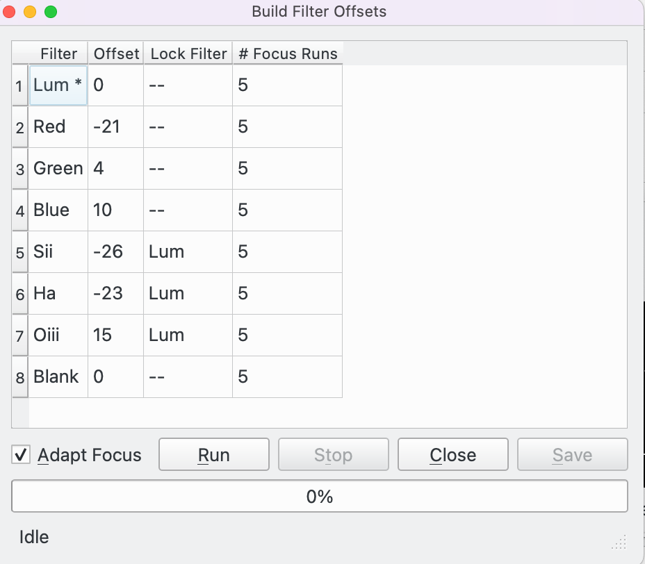 |
Click the Build Offsets button on the Filter Settings popup to launch the Build Offsets tool. Filter Offsets can either be entered manually into the table in the Filter Settings popup or this tool can be used to assist in creating them.
Note: This utility should not be run during an imaging session as it takes exclusive control of the Focus process whilst it is running.
To start with, configure settings for each filter in the table in the Filter Settings popup and then launch Build Filter Offsets. The popup is launched with a table of data with the following columns.
Filter: Filter Name. The first filter has an "*" after the filter name, "Lum *" in the above example. This means that Lum is the reference filter against which offsets for other filters will be measured. Double click another Filter Name to make that filter the reference filter.
Offset: The current offset.
Lock Filter: The current Lock filter.
# Focus Runs: The number of focus runs for this filter. The default is 5. To exclude a filter from the process set this field to zero. Note, the reference filter must have at least 1 run.
When the # Focus Runs have been configured press the Run button to start the automated process.
Press the Stop button to stop the process at any time.
Toggle the Adapt Focus checkbox at any point in the processing to switch between measured Autofocus results and results after Adaptive Focus adjustments have been applied. See the Adaptive Focus section for more details on what Adaptive Focus is.
Let's take an example where we have 7 filters: Lum, Red, Green, Blue, Sii, Ha and Oiii. The 8th slot in the filter wheel is marked as Blank. The process has completed 5 runs for all filters, 0 for Blank (effectively excluding Blank from the process). In this case 8 extra columns have been created in the table.
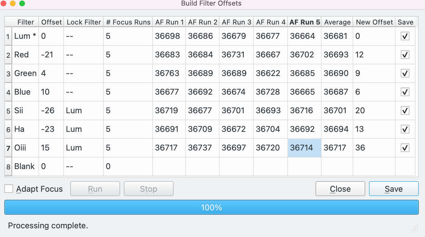 |
AF Run 1-5: The maximum # Focus Runs selected by the user is 5, so 5 columns have been created, 1 for each AF run solution.
Average: The average (mean) of the AF solutions.
New Offset: The offset calculated from the Lum filter. E.g. for Sii 36731 - 36743 = -12
Save: Check to save the offset for this filter when the Save button is pressed. The default is to check these boxes but unchecking allows a value to be ignored whilst saving other filters.
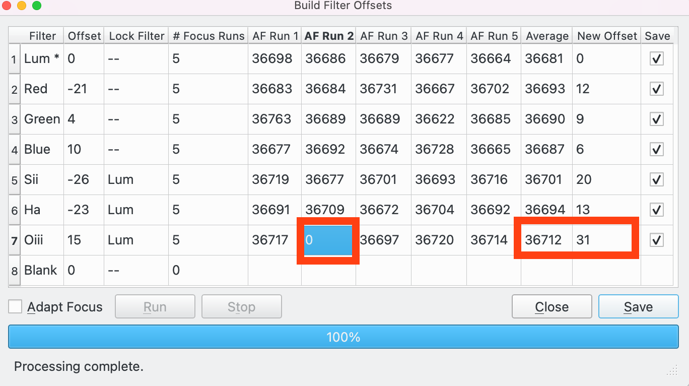
At this stage, it is recommended to review the AF runs to make sure they are all good. For example, lets assume we are unhappy with the 2nd AF run on Oiii. In this case we could either:
Edit AF Run 2 and set the value to whatever value we want.
Edit the New Offset column and set the value directly (bypassing the logic to calculate it).
Discard the AF Run 2 by setting the value to 0 (see below). In this case, the Average and New Offset for Oiii is recalculated based on AF Runs 1, 3, 4, 5. In the example below the new Average and New Offsets are calculated and displayed.
 |
After reviewing the results, the user can press:
Save: All filters where the Save checkbox is checked will have the New Offset value saved in Filter Offsets for use during the next imaging session.
Close: The Build Filter Offsets tool is closed without saving any data.
If the Adapt Focus box is checked, the AF Runs are updated for Adaptive Focus. See the Adaptive Focus section for more details on the theory of Adaptive Focus. The first AF run (in this example AF Run 1 on Lum) is the basis for the Adaptations. So the temperature and altitude of AF Run 1 on Lum is used as the basis for all the other AF Runs and the data is adapted back to what the AF solution would have been, had it been run at the temperature and altitude of AF Run 1 on Lum.
In this example, Adaptive Focus is setup for Altitude adjustments on the Red filter only in Filter Settings. So the Adapted AF Run values are the same as the unadapted values for all the other filters.
 |
If you hover the mouse over an AF Run it will show a tooltip Adaptive Focus Explainer. In the example, the mouse is hovering over AF Run 1 on Red. The 1st row of the Explainer shows the measured Autofocus result for that run (36683), adaptations for Temperature (0.0C) and Altitude (0.2 degrees Alt). The 2nd row of the Explainer shows the Adaptations: 206 total, 0 temperature, 205.9 altitude. The 3rd row shows the Adapted Position of 36889.
The user can toggle between Adapt Focus or raw values. Whichever values are displayed in the grid will be the values that are saved.
Here are some tips for using this utility:
Start by making sure the area of the sky you are running Build Filter Offsets on works well for Autofocus. Aiming high in the sky will result in shooting through less atmosphere with smaller, tighter stars. Make sure there are enough stars in the frame. Avoid Meridian Flips during the process. Track the same area during the process so each run is using more or less the same set of stars. Although the facility to use Adapt Focus is available to adjust for environmental changes such as temperature and altitude try to minimise these changes over the course of running the utility by selecting an appropriate area of the sky.
Make sure your equipment is in thermal equilibrium before starting. Calculate roughly how long the utility will take which is the total number of AF runs * time for a single AF run. Try to make sure that the conditions will remain as consistent as possible during this time, e.g. there is enough time before dawn, the moon won't affect focusing of some images more than others, the target won't drop below your horizon during the process, etc.
Configure the utility for # Focus Runs (5 is a good start), reference filter (e.g. Lum) and Adapt Focus setting. Run the utility to completion.
Review the results. For each filter review each AF run looking for outliers. For each outlier decide what to do, e.g. remove from processing by setting to 0. If there are filters for which you are unhappy with the results, uncheck the Save checkbox for those filters.
When happy, press Save to save the filter offsets to Filter Settings for future use.
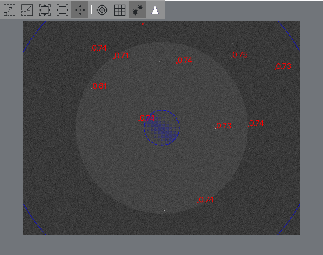 |
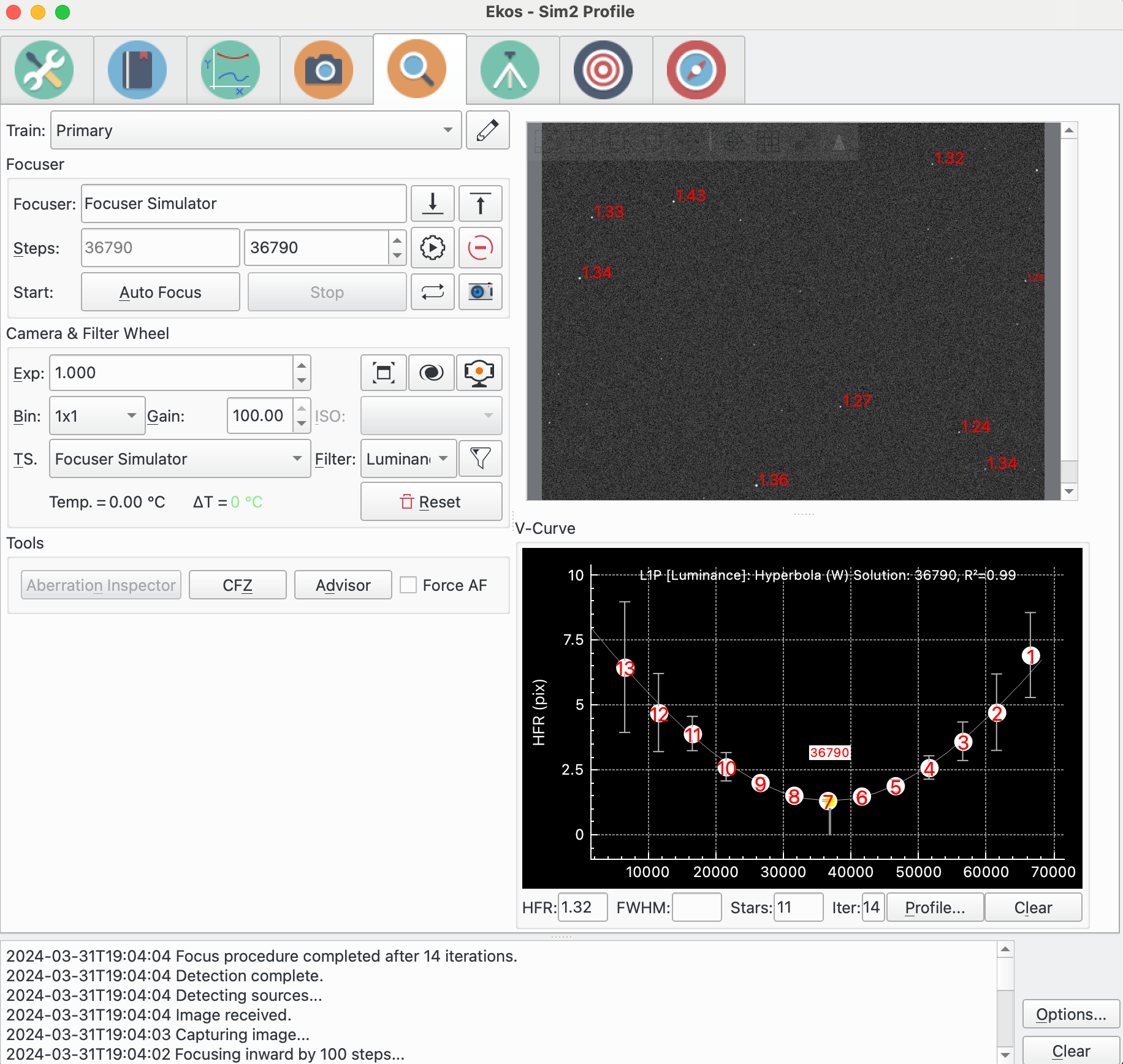
The focus display, displays a FITS viewer window onto the frame taken during the focus process. If Ring Mask is selected, then the mask is drawn on the image. All the stars detected by Ekos based on the selected parameters, have their HFR value displayed next to the associated star (unless Measure is set to FWHM).
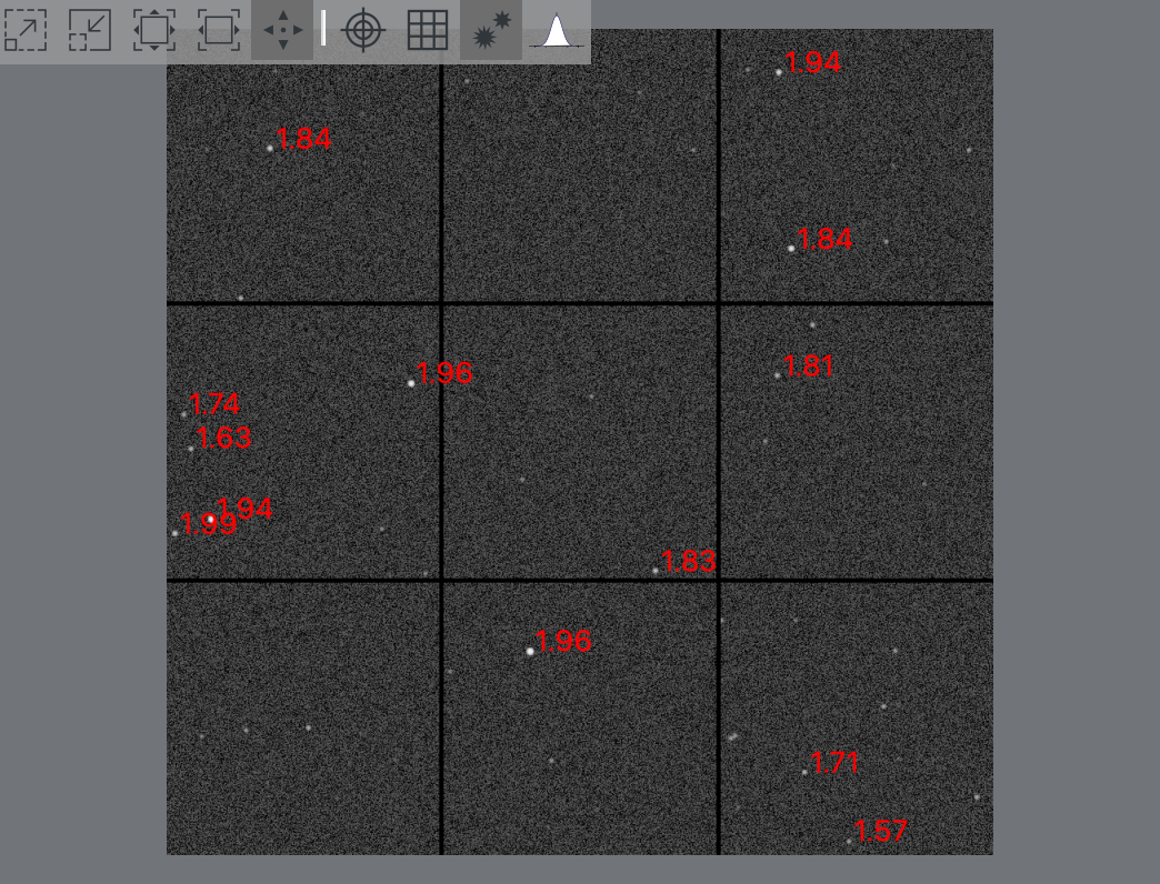
If Mosaic Mask has been selected then the FITS viewer displays the mosaic 3x3 grid showing the center, edges and sides as configured in the Mosaic Mask options.
 |
The window supports the following FITS viewer options (at the top of the window):
and .
and .
: Toggle screen stretch on or off.
: Toggle crosshairs on or off.
: Toggle pixel gridlines on or off.
: Toggle star detection on or off.
: Launches the View Star Profile dialog.
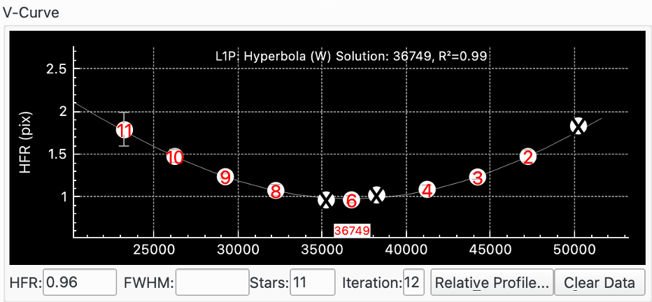 |
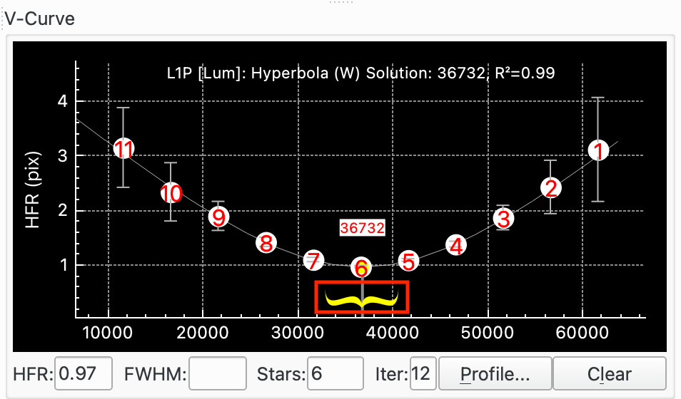
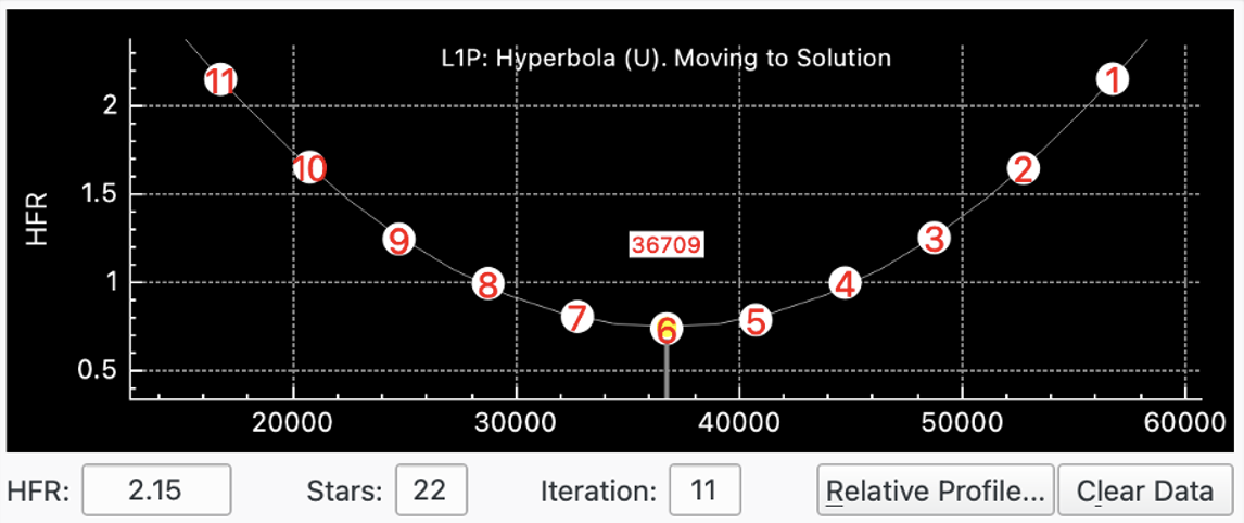
The V-Curve displays focuser position (x-axis) versus focus Measure, e.g. Half-Flux-Radius (HFR) (y-axis). Each datapoint is drawn on the graph and represented by a circle with a number representing the datapoint. How many datapoints are taken and how the focuser moves is determined by the parameters chosen.
For certain algorithms, Ekos will also draw a curve of best fit through the datapoints. If Use Weights is selected then error bars are indicated on each datapoint that correspond to the standard deviation in measured value.
The units of the y-axis depend on the selected focus Measure. For example, for HFR, the y-axis will either be in Pixels or Arc seconds depending on how Display Units is set.
If Refine Curve Fit is selected, Focus will check for and potentially exclude outlying datapoints. In this case datapoints 1, 5 and 7 were excluded.
Under the V-Curve a number of parameters are displayed:
HFR: Displays the star HFR for the most recent datapoint if relevant.
FWHM: Displays the star FWHM for the most recent datapoint if relevant.
Stars: The number of stars used for the most recent datapoint.
Iteration: The number of datapoints taken so far.
: Invokes the Relative Profile popup.
: Resets the V-Curve graph by clearing the displayed data.
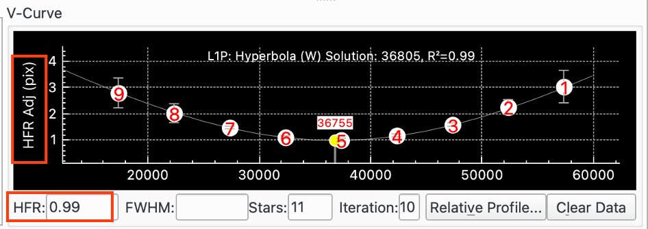
Here is a V-Curve when Measure is set to HFR Adj:
 |
Here is a V-Curve when Measure is set to FWHM:
 |
Here is a V-Curve when Measure is set to # Stars. In this case the Critical Focus Zone (CFZ) Display checkbox has been checked so the CFZ is displayed as well:
 |
Here is a V-Curve when Measure is set to Fourier:
 |
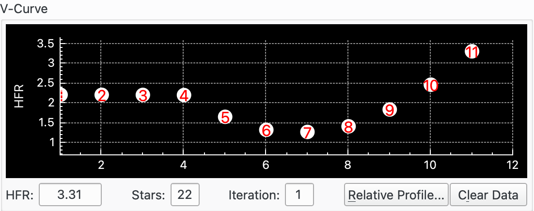
When Framing, the graph format changes to that of a "time series" where horizontal axis denotes the frame number. This is to aid you in the framing process as you can see how Measure, in this case HFR, changes between frames.
This is very useful, for example, when trying to get the system into approximate focus before starting an Autofocus run. In this case Framing is started and the Step In and Step Out buttons used to adjust focus and the effect on the V-Curve observed.
 |
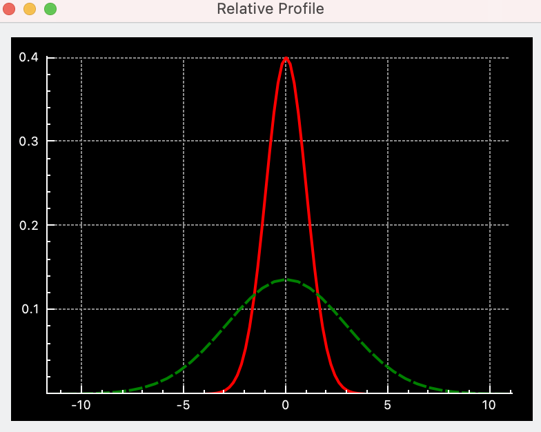 |
The relative profile is a graph that displays the relative HFR values plotted against each other. Lower HFR values correspond to narrower shapes and vice-versa. The solid red curve is the profile of the current HFR value, while the dotted green curve is for the previous HFR value. Finally, the magenta curve denotes the first measured HFR. This enables you to judge how well the Autofocus process improved the relative focus quality.
The exact settings that work best for a given astronomical setup need to be worked out by the user using trial and error. A good place to start is the Focus Advisor section. Run Focus Advisor and accept its recommendations. It uses the Linear 1 Pass algorithm:
Setup Backlash. See the Backlash section for more details.
Initial Step Size. This is a critical parameter. You may have an idea from other people with a similar setup. If not you can try setting it from the Critical Focus Zone (CFZ) for your equipment. See the CFZ section for more details.
Start near to focus by manually finding focus. Use the option and manually adjust the focus to get to approximate focus.
Make sure you are finding enough stars. Increasing the exposure usually finds more stars (but makes the focus process longer).
Run Autofocus. This is the sort of V-Curve you are after:
 |
In contrast, the next picture shows an Initial Step Size that has been set too low. The HFR varies from about 0.78 to 0.72. Which gives a max / min just over 1. The other clue that this is a poor setup is that the Error Bar range is very large compared to HFR movement which means that the curve solver is drawing a curve through a lot of noise, which means the results will not be very accurate.
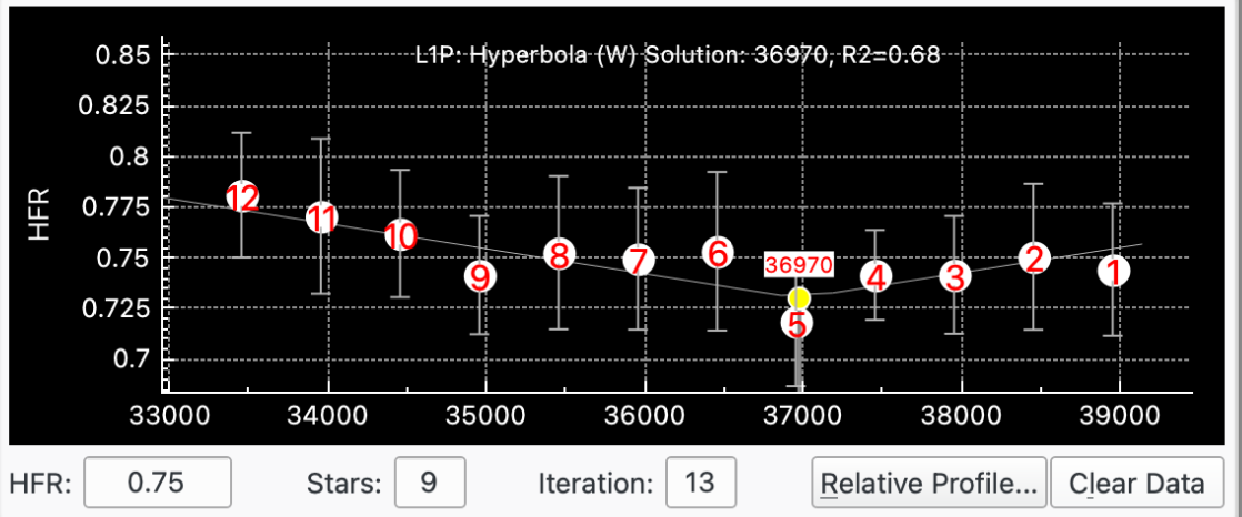 |
Backlash in the focuser setup is due to a combination of backlash in the electronic focuser itself (e.g. in the gearing mechanism), in the binding of the electronic focuser to the telescope drawtube, and in the telescope drawtube's mechanism. Thus, each setup will have its own backlash characteristic even if the same focuser is used.
It is important to have a clear strategy for dealing with Backlash and to setup Focus appropriately for the chosen strategy. It is best to have backlash managed in one place to avoid conflicts. Whilst it is possible to have backlash managed in multiple places (this has been done successfully) it is not recommended in general because it can lead to conflicts between software components and the focuser.
There are several ways to measure backlash in ticks. Consult the documentation on your focuser or use the internet including the Indi Forum.
There are several things to consider when working out how to deal with backlash:
No Backlash: If you are fortunate enough to have a setup with no backlash then it would make sense to set Driver Backlash and AF Overscan off (set to zero).
Backlash Managed by Focuser: If your focuser had the ability to manage backlash itself then you can use this facility and turn Driver Backlash and AF Overscan off (set to zero). Alternatively, if it's possible, you could turn off the focuser's backlash facility and use either the Device Driver or AF Overscan to manage backlash.
Backlash Managed by Device Driver: If your device driver has the ability to manage backlash then you can use this facility and turn off AF Overscan (set to zero). Alternatively, you could turn off the device driver's backlash facility and set AF Overscan.
To know whether the device driver supports backlash, check the Driver Backlash field. If it is enabled and you can set values then the driver supports Backlash. If the field is disabled then the driver does not support Backlash.
AF Overscan: The Focus module can manage Backlash itself by over scanning outward motions by the value in the AF Overscan field. For example, if AF Overscan is set to 40 then whenever Focus moves the focuser outwards, it does this as a 2-step process. Firstly it moves the focuser 40 ticks past where it wants to end up; secondly it moves back in by 40 ticks.
The advantage of AF Overscan is that you do not need to know Backlash exactly, you just need to set the AF Overscan >= backlash. So, for example, if you measure backlash as around 60 ticks then you could set AF Overscan to 80.
AF Overscan is also useful where Backlash is not exactly predictable. For example, if Backlash measurements yield slightly different values, e.g. 61, 60, 59 ticks then by using AF Overscan this inconsistency can be effectively neutralised. Were you to use Focuser Backlash you would probably average the readings and set the value to 60. Sometimes this will correctly take up all the backlash; sometimes it will be a little short; and sometimes it will over correct.
All focuser movements managed by Focus will have AF Overscan applied, including Step Out, Goto, Autofocus runs, Adaptive Focus movements, Adapt Start Pos movements and Take flats at the same position as lights.
 |
Ekos supports the concept of Adaptive Focus (AF). Without AF, a typical imaging plan would start with an Autofocus run then a sequence of subframes, then an Autofocus run, etc. The Autofocus runs would be triggered by a number of factors such as time, filter change, temperature change, etc. So basically as a sequence runs subframes are being taken slightly away from optimum focus until a threshold (e.g. temperature change) triggers an Autofocus run.
The idea of AF is to adjust focus as environmental factors change to try to take each subframe as close as possible to optimum focus. Ideally, the effect of Adaptive Focus is like performing an Autofocus run before each subframe but without the overhead of actually doing the run.
AF works as a complement to the various triggers for Autofocus that are available in Ekos now. So it is not necessary to change the Autofocus triggers when starting to use AF. Indeed, at the start, it is not recommended to relax Autofocus conditions when using AF. However, over time, as confidence grows in AF it would be possible to do less Autofocusing (and therefore more imaging). But either way, each subframe should be more in focus when using AF, providing it is setup correctly.
So how do you know if AF would be useful for your setup or not? Perhaps the simplest way would be to examine subframes just after an Autofocus and compare them with subframes just before the next Autofocus. Can you see a difference in focus? If you have a setup where the focus point is tolerant of environmental changes between Autofocus runs then AF may not add anything to your images; if however you have a setup that is sensitive to environmental changes and the frequency of Autofocus runs is a compromise between quality and imaging time then AF ought to improve the quality of your subframes.
AF currently supports two environmental dimensions: Temperature and Altitude (of the imaged target):
Temperature. All the components of the imaging system will be affected by changes in ambient temperature. The most obvious will be the telescope tube. Typically this will expand as temperature increases and contract as it decreases. This will affect the focus point. But also the optical path the light from the imaged target takes through the atmosphere and through the imaging components of the telescope will be affected by temperature and therefore will affect the focus point.
It is necessary to have a reliable source of temperature information available to the focus module in order to use the temperature feature of AF.
Where the temperature source is located is, of course, up to the user. Given the changes in temperature effect many components it is not obvious where the best location would be. Some experimentation may be required to get the best results but as a guide, the source should be near the imaging train but not near any heating effect of electrical equipment that would say, heat the temperature source but not the optical train. Consistency of location is likely to be important.
Altitude. Some users have reported that the focus point changes with the altitude of the target. This effect is likely to be smaller than the temperature effect and may be negligible for some setups.
To use AF you need to work out firstly whether you want to adapt for Temperature, Altitude or both. If you are new to AF it is recommended to start with Temperature and once you have that working, determine whether your setup would benefit from adding Altitude.
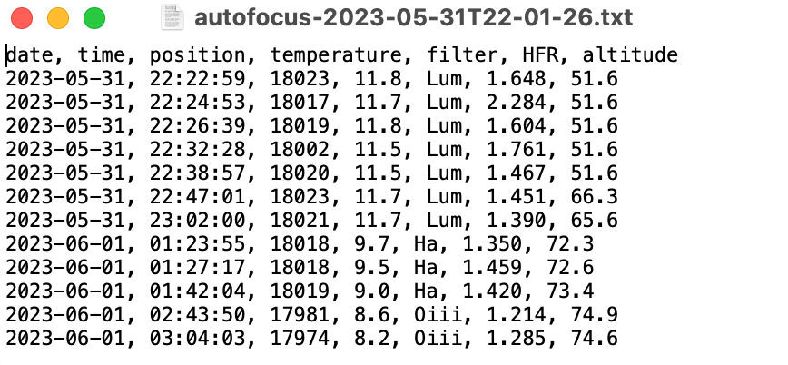
The first step is to workout the Ticks / °C and/or Ticks / °Alt for your equipment. To do this there is an existing utility in Ekos whereby when Focus logging is enabled, in addition to adding focus messages to the debug log, every time an Autofocus run completes, information is written to a text file in a directory called focuslogs located in the same place as the debug logs directory. The files are called “autofocus-(datetime).txt”. The data written are: date, time, position, temperature, filter, HFR, altitude. This data will need to be analysed outside of Ekos to determine the Ticks / °C and if required the Ticks / °Alt.
Here is an example of a “autofocus-(datetime).txt” file:
 |
Currently Ekos supports a simple linear relationship between temperature, or altitude, and ticks. In the future, if there is demand, more sophisticated relationships could be supported. A linear relationship will deliver the majority of the benefit of AF and is fairly straight-forward to administer. More complex relationships could be more accurate but come with more complex administration. Note also that more complex focus point vs temperature relationships will likely be more or less linear for small changes in temperature.
A way to get a value for Ticks / °C would be to take the data from the autofocus-(datetime).txt files from a few nights of observing into a spreadsheet and graph focus position against temperature for each filter. Review the data and remove any outliers and plot a line of best fit. Use the line to get Ticks / °C. If you intend to adapt for altitude as well as temperature, then it would be better to use a set of data at similar altitude when calibrating temperature. Then it's possible to calculate the effect of Temperature and remove this from the data when calculating the effect of Altitude.
You will need to ensure that your focus position is repeatable at the same temperature and altitude and that there is no slipping of the focuser or uncompensated backlash. In addition, when calibrating it is better to avoid changing the optical train in a way that could change the focus position. If this is unavoidable and if the change affected the focus position then you will need to appropriately adjust the historical focus data so they can be compared.
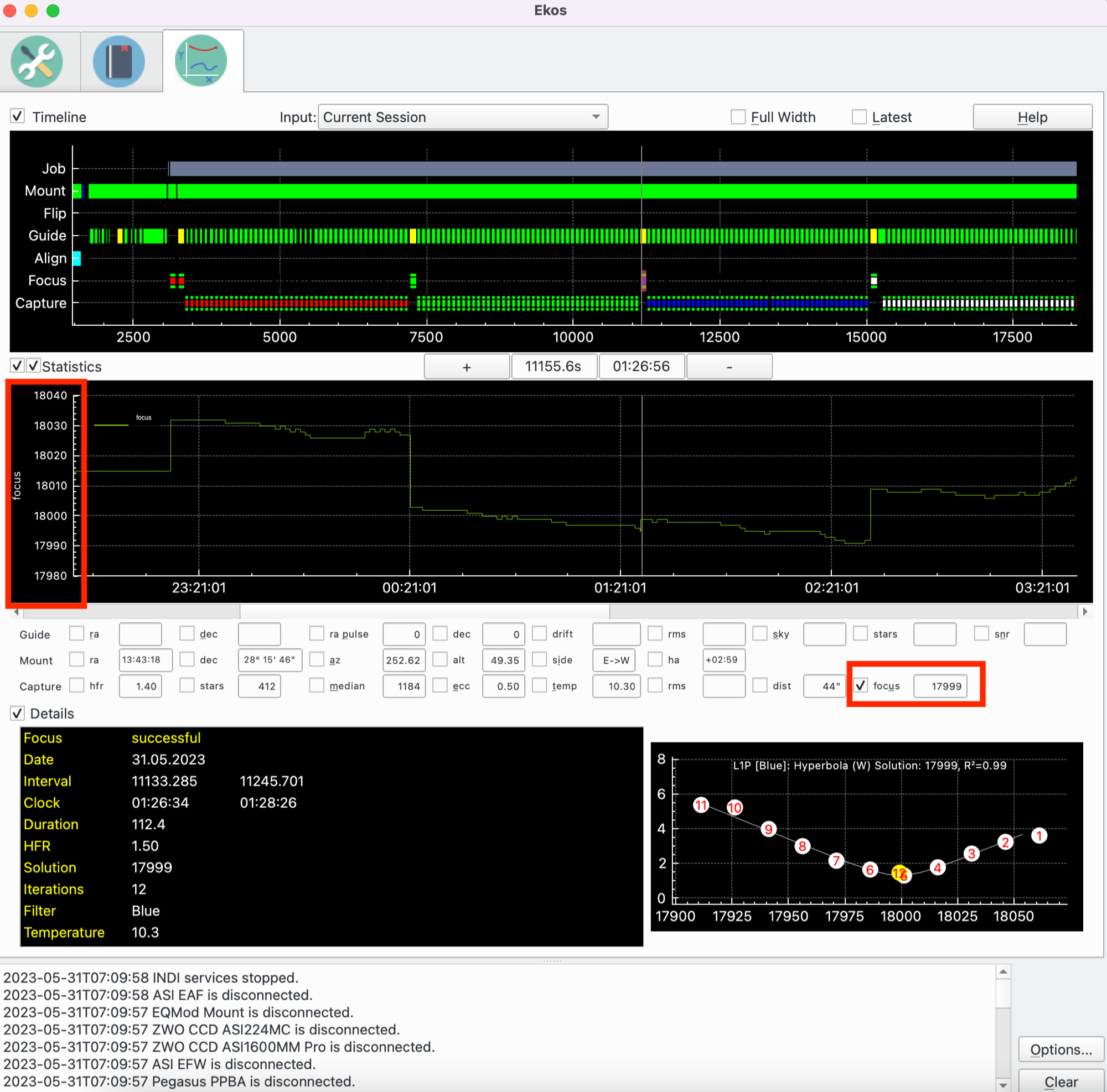
A simple approach is to start with a small amount of data, say 1 night and use this to calculate, say the Ticks / degree C. Run with this and adjust it over time as you collect more data. A way to check how well AF is performing would be to use Analyze to review how AF had moved the focus over 1 hour. If things are spot on, then where ever AF had positioned the focuser after 1 hour would match the Autofocus result. Where there is a discrepancy, it will be because of randomness in the Autofocus result and miscalibration in the AF Ticks / °C. By doing this regularly you will build knowledge of your equipment and be able to fine tune AF. Below is a screenshot of Analyze configured for Focus where you can see how Focus position changes throughout the imaging session:
 |
Once you have your data you can configure it in the Filter Settings popup. Then in Focus, switch on Adaptive Focus in Focus Settings. At this point, when you run a sequence, Ekos will check after each subframe whether it needs to adapt the focuser position. If so, Focus will do that and then Capture will continue with the next Subframe.
The screenshot at the top of this section shows an example. Ticks / °C is set to 9. Autofocus ran and it solved at 36580 at 10C. Then a simple sequence of 5 subframes was run. The temperature was firstly set to 9C then to 8C. After each subframe completed, Ekos performed an adaptive focus run and where there was a temperature change it calculates the number of ticks to move the focuser. In this example, the focuser was moved inward by 9 ticks on 2 separate occasions, starting at 36580, before moving to 36571 and then to 36562 as shown on the Focus Tab in the Current Position widget and in the message box.
The Adaptive Focus concept has been built into the Build Offsets tool.
The Coefficient of Determination, or R², is calculated in order to give a measure of how well the fitted curve matches the datapoints. More information is available here. This feature that is available for the Linear 1 Pass focus algorithm. In essence, R² gives a value between 0 and 1, with 1 meaning a perfect fit where all datapoints sit on the curve, and 0 meaning that there is no correlation between the datapoints and the curve. The user should experiment with their equipment to see what values they can obtain, but as a guide, a value above, say 0.9 would be a good fit.
There is an option to set an “R² Limit” in Focus Settings that is compared to the calculated R² after the auto focus run has completed. If the limit value has not been achieved, then the auto focus is rerun.
Setting an R² Limit could be useful for unattended observation if the focus run produces a bad result for a 1-off reason. Obviously if the reason is not transitory then rerunning will not improve anything.
If the R² Limit is not achieved and the focus process is rerun, and again fails to achieve the R² Limit, then the focus run is marked as successful to avoid the process getting stuck rerunning auto focus forever.
This feature is turned off by setting the R² Limit to 0.
The Levenberg-Marquardt (LM) algorithm is used to solve non-linear least squares problems. The GNU Science Library provides an implementation of the solver. These resources provide more details:
The Levenberg-Marquardt algorithm is a non-linear least-squares solver and thus suitable for many different equations. The basic idea is to adjust the equation y = f(x,P) so that the computed y values are as close as possible to the y values of the datapoints provided, so that the resultant curve fits the data as best as it can. P is a set of parameters that are varied by the solver in order to find the best fit. The solver measures how far away the curve is at each data point, squares the result and adds them all up. This is the number to be minimized, let's call it S. The solver is supplied with an initial guess for the parameters, P. It calculates S, makes an adjustment to P and calculates a new S1. Provided S1 < S then we are moving in the right direction. It iterates through the procedure until:
the delta in S is less than a supplied limit (convergence has been reached), or
the maximum number of iterations has been reached, or
the solver encountered an error.
The solver is capable of solving either an unweighted or weighted set of datapoints. In essence, an unweighted set of data gives equal weight to each datapoint when trying to fit a curve. An alternative is to weight each datapoint with a measure that corresponds to how accurate the measurement of the datapoint actually is. In our case this is the variance of star HFRs associated with the datapoint. The variance is the standard deviation squared.
Currently the solver is used to fit either a parabolic or a hyperbolic curve.
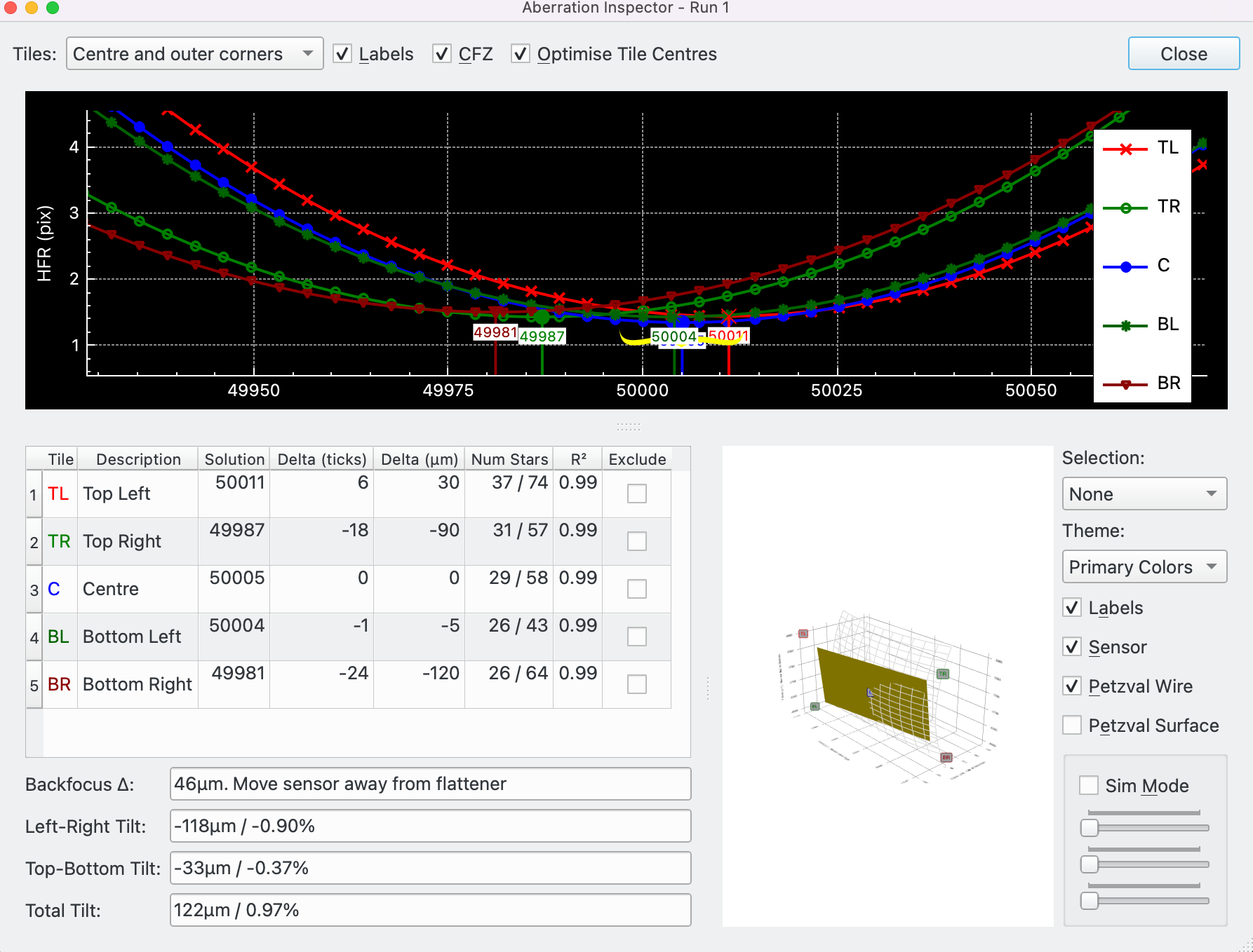 |
The Aberration Inspector is a tool that makes use of Autofocus to analyze backfocus and sensor tilt in the connected optical train.
To run Aberration Inspector press the button. See Focus Tools for more details. The following criteria must be met in order for the button to be active and the tool to work:
The focuser must be an absolute focuser.
The focus algorithm must be Linear 1 Pass.
A mosaic mask must be applied.
Focuser step size needs to be setup. It is the number of microns the focal plane moves for 1 focuser tick. This is setup in the CFZ dialog. See the CFZ section for more details.
When the Inspector button is pressed, AutoFocus will run, but in addition, for each datapoint, extra information is captured for later use by Aberration Inspector. Once Autofocus completes, the Aberration Inspector dialog is displayed.
To initially setup to use the tool it is recommended to do the following:
Point to a part of the sky where Autofocus solves well. Typically this would be high in the sky away from any obstacles. Choose somewhere with lots of stars such as the Milky Way. The reason this is more important for Aberration Inspector than Autofocus is that focus analysis needs to be performed for each tile in the mosaic. Therefore, it is important that each tile has enough stars to perform accurate Autofocus.
Run Autofocus a couple of times to ensure it is solving correctly and that you have a good set of stars in each mosaic tile. Whilst most focus parameters can be used it is recommended to use the parameters that work best for Autofocus with your equipment. The reason for this is that Aberration Inspector needs be focus solve each mosaic tile and not just the sensor as a whole.
A mosaic mask must be applied. Some experimentation will be required to set this up optimally for your equipment. The configuration parameter to adjust is the tile size which is the size of tile as a percentage of sensor width. The higher the percentage, the bigger each tile, e.g. for a 4:3 sensor using a tile size of 25% means each tile is 8% of the sensor's area. Using a tile size of 10% means each tile is 1% of the sensor's area. The bigger the area the more stars will be present and the better the focus algorithm will solve. However, the purpose of the Aberration Inspector is to provide information on aberrations (backfocus and tilt) across the sensor, so ideally the information for each tile would be specific to as small an area as possible.
The sweet spot for tile size is as small a value as possible that still contains enough stars to solve well in each tile.
The Aberration Inspector can be used in conjunction with a device to adjust tilt and / or backfocus. The method to do this is an iterative approach, like for example, collimating a telescope. The steps are:
Run the Aberration Inspector and obtain results.
Inspect the results and make sure they are good, e.g. number of stars in each tile is sufficient and the R² is acceptable for all relevant tiles.
Adjust tilt and / or backfocus using your device, based on Aberration Inspector results.
Re-run Aberration Inspector. It will launch another dialog. Check results as before. If the tilt and / or backfocus is getting better then the adjustment was made in the correct sense; if not reverse the sense and retry. Use the feedback from the previous adjustment for the next adjustment.
Repeat the above process until the limit of sensitivity of the equipment is reached.
Note the amount of adjustment, e.g. how far to turn bolts, and the sense, clockwise or counter-clockwise, will vary by equipment and must be discovered by the user by trial and error. Always follow the recommendations of the tilt / backfocus device manufacturer.
Each time Aberration Inspector is run it launches a new dialog with the run number appended to the title. This way several runs can be performed and the results compared. Note, however, that the dialog holds a lot of data (roughly 10x the amount of a standard Autofocus run). The system resources associated with this are released when the dialog is closed. For this reason on lower powered machines, once the tool has been used, it is recommended to close all Aberration Inspector dialogs before imaging.
The following sections describe the sections of the Aberration Inspector dialog.
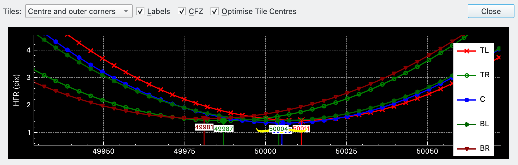 |
At the top of the dialog are some controls, followed by the V-Curve. The controls are:
Tiles: Three options are available:
All: All 9 tiles are displayed.
Centre and outer corners: The centre and 4 corner tiles are displayed.
Centre and inner diamond: The centre and 4 inner diamond tiles are displayed.
Labels: Checkbox toggles focus point labels on the V-Curve.
CFZ: Checkbox toggles whether the CFZ moustache is displayed on the V-Curve.
Optimise Tile Centres: If unchecked, the geometrical centre of the tile is used; if checked, the centre of the tile is calculated as an average of the star positions within the tile. Whilst theoretically more accurate to check this option, it is likely to have a significant impact only if the number of stars is small.
Close: Close the Aberration Inspector dialog.
The V-Curve is similar to the V-Curve on the main Focus tab, except each tile is represented by its own curve. The number of curves is determined by the setting of the Tiles combobox. The x-axis displays the focuser position and the y-axis the measure (e.g. HFR) used by Autofocus. Each curve has its own colour and 2 character identifier as displayed in the legend.
Hover the mouse over a curve minimum to see more information about that curve.
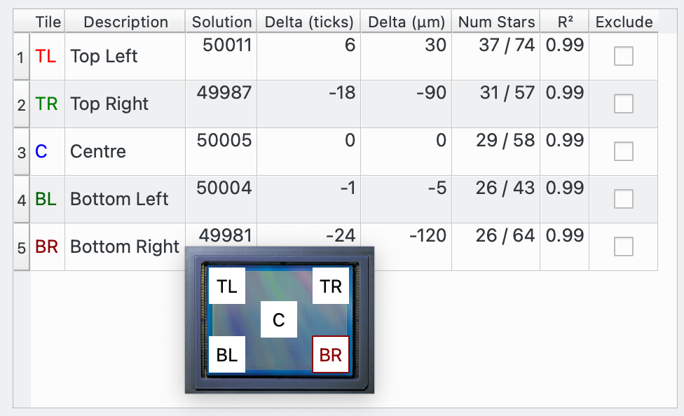 |
The table displays information pertinent to each tile as selected by the Tiles setting.
A tooltip like graphic is displayed when the mouse is hovered over either of the leftmost 2 columns. The graphic displays a picture of the sensor scaled to the dimensions of the sensor. Overlayed on the sensor are the tiles as selected by the Tiles setting. The tiles are scaled appropriately for the tile settings. Each tile is labelled with the Tile Name and the tile corresponding to the row that the mouse is hovering over, is highlighted in the colour of that tile.
The following columns are displayed:
Tile: The 1 or 2 character name of the tile, e.g. TL = Top Left, C = Centre, etc.
Description: Tile Description, e.g. Top Left, Centre, etc.
Solution: The focus solution. This matches the solution on the V_Curve.
Delta (ticks): This is the delta of the solution for the current table row from the solution of the Centre tile. The Delta of the Centre row will, of course, be zero.
Delta (μm): This is Delta (ticks) converted to microns using the step size in microns as specified in the CFZ Focus tab.
Num Stars: This shows the min / max number of stars detected during the Autofocus run. Usually, the minimum number would be a far out of focus datapoint and the max number would be the in focus datapoint.
R²: R-squared of the curve fit for this tile. See Coefficient of Determination for more details.
Exclude: Checkbox to include / exclude this tile in calculations. By default, if a tile has been curve fitted it will be included; if a tile was not curve fitted then it will be excluded. In addition, the user may decide that a particular tile may contain poor quality data, for example the R² is low; or the number of stars is low. In this case the Exclude can be checked and this row will be excluded from calculations. Note that by excluding some rows, some calculations may not be performed. If the Centre tile is excluded, no calculations can be performed.
Note that whilst it's possible to exclude tiles and still get calculated values, if the data is poor quality then it is recommended to rerun Aberration Inspector rather than persist with poor quality data.
The recommended approach is to check the table for quality data and once achieved, move onto analysing the Aberration Inspector Results.
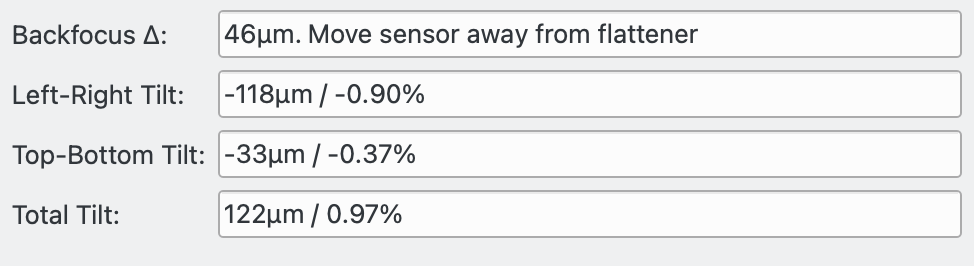 |
The calculation results are displayed in this section, based on the data displayed in the table:
Backfocus Δ: This is the value of the Backfocus delta. The nearer to perfect backfocus, the lower the backfocus delta. Note that the Backfocus delta gives a clue as to how far out the Backfocus is, in terms of scale and direction, but is not the amount by which the sensor needs to be moved. The relationship between backfocus Delta and how far to move the sensor will vary with the equipment used, and needs to be worked out by the user.
The field gives the sense of the backfocus movement required to improve backfocus: either move the sensor nearer to the field flattener (telescope) or move it further away.
Left-Right Tilt: Gives the Left to Right tilt in microns and as a percentage.
Top-Bottom Tilt: Gives the Top to Bottom tilt in microns and as a percentage
Total Tilt: The diagonal tilt in microns and as a percentage.
The smaller the backfocus delta the nearer the sensor is to perfect backfocus. If the field flattner does not flatten the field all the way to the edges of the sensor then this will be visible by switching the Tiles option between "Centre and outer corners" and "Centre and inner diamond". If the backfocus delta results are consistent when the Tiles option is changed then this indicates that the field flattener is working to the corners of the sensor.
There will always be some backfocus delta at least because of noise in the observation data. The important thing is that when in focus, stars are circular in all parts of the sensor.
The smaller the tilt percentages, the nearer the sensor is to being flat to the plane of light from the flattener / telescope. As with backfocus delta, there is always going to be some noise in the data, which will present as tilt. The important thing is that when in focus the star sizes are consistent across all parts of the sensor.
Because of the nature of the backfocus delta and tilt calculations, one will affect the other so it will probably be better to try and adjust both together, in small increments, rather than trying to perfect one in isolation, before adjusting the other.
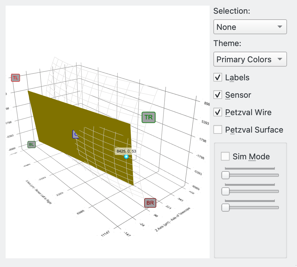 |
The 3D graphic displays the sensor tilted as per the Aberration Inspector Results. To help visualise the Petzval surface (see Petzval Field Curvature for more details) of light coming out of the telescope and incident on the sensor the surface is also modelled. The higher the backfocus error, the more curved the Petzval surface.
The graphic can be zoomed and rotated using gestures. To zoom use pinch. To rotate use touch-and-move.
The graphic has a Simulation Mode that allows backfocus and tilt to be adjusted by the sliders. The effect on the sensor's tilt and Petzval surface is displayed in the graphic.
The following options are available for the graphic:
Selection: The following options are available:
None: No selection is possible.
Item: A datapoint may be selected and data values are displayed.
Slice: A 2D slice through the 3D graphic is displayed.
Theme: A number of colour themes are available.
Labels: Checkbox to show / hide tile labels on the graphic.
Sensor: Checkbox to show / hide the sensor.
Petzval Wire: Checkbox to show / hide the Petzval surface as a graphic wire.
Petzval Surface: Checkbox to show / hide the Petzval surface.
Sim Mode: Checkbox to toggle Simulation Mode on / off. When off, the graphic displays the sensor and Petzval surface based on the calculated results of the Aberration Inspector run. When on, the sliders for Backfocus, Left-to-Right tilt and Top-to-Bottom tilt are activated, and these can be dragged by the user to adjust the graphic. Hover the mouse over each slider to see the tooltips describing what each slider does.
The 3D graphic is not essential to using Aberration Inspector. All relevant information is displayed in the Table and Results sections of the dialog. Its purpose is to aid the user in understanding Aberration Inspector and to orient themselves with the information the tool provides.