Table of Contents
KmPlot deals with several different types of functions, which can be written in function form or as an equation:
Cartesian plots can either be written as e.g. “y = x^2”, where x has to be used as the variable; or as e.g. “f(a) = a^2”, where the name of the variable is arbitrary.
Parametric plots are similar to Cartesian plots. The x and y coordinates can be entered as equations in t, e.g. “x = sin(t)”, “y = cos(t)”, or as functions, e.g. “f_x(s) = sin(s)”, “f_y(s) = cos(s)”.
Polar plots are also similar to Cartesian plots. They can be either be entered as an equation in θ, e.g. “r = θ”, or as a function, e.g. “f(x) = x”.
For implicit plots, the name of the function is entered separately from the expression relating the x and y coordinates. If the x and y variables are specified via the function name (by entering e.g.“f(a,b)” as the function name), then these variables will be used. Otherwise, the letters x and y will be used for the variables.
Explicit differential plots are differential equations whereby the highest derivative is given in terms of the lower derivatives. Differentiation is denoted by a prime ('). In function form, the equation will look like “f''(x) = f' − f”. In equation form, it will look like “y'' = y' − y”. Note that in both cases, the “(x)” part is not added to the lower order differential terms (so you would enter “f'(x) = −f” and not “f'(x) = −f(x)”).
All the equation entry boxes come with a button on the right. Clicking this invokes the advanced Equation Editor dialog, which provides:
A variety of mathematical symbols that can be used in equations, but aren't found on normal keyboards.
The list of user constants and a button for editing them.
The list of predefined functions. Note that if you have text already selected, it will be used as the function argument when a function is inserted. For example, if “1 + x” is selected in the equation “y = 1 + x”, and the sine function is chosen, then the equation will become “ y = sin(1+x)”.
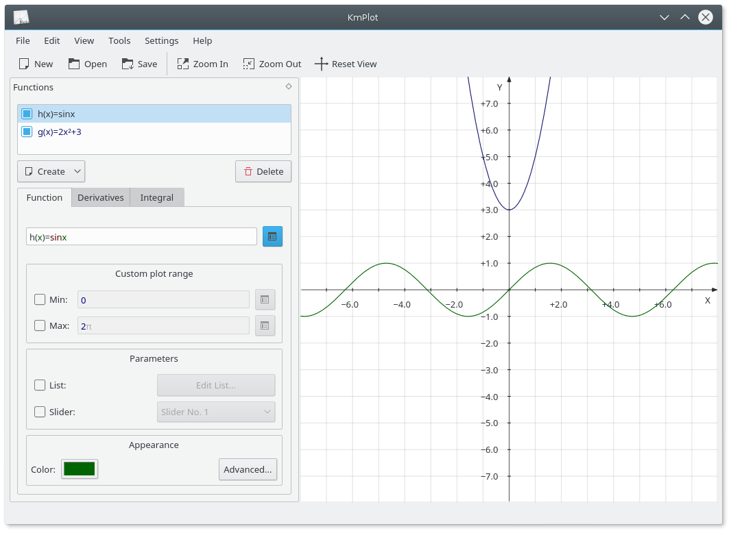
To enter an explicit function (i.e., a function in the form y=f(x)) into KmPlot, just enter it in the following form:
f(x) = expressionwhere:
fis the name of the function, and can be any string of letters and numbers.xis the horizontal coordinate, to be used in the expression following the equals sign. It is a dummy variable, so you can use any variable name you like to achieve the same effect.expressionis the expression to be plotted, given in the appropriate syntax for KmPlot. See the section called “Mathematical Syntax”.
Parametric functions are those in which the x and y coordinates are defined by separate functions of another variable, often called t. To enter a parametric function in KmPlot, follow the procedure as for a Cartesian function for each of the x and y functions. As with Cartesian functions, you may use any variable name you wish for the parameter.
As an example, suppose you want to draw a circle, which has parametric
equations x = sin(t), y = cos(t). After creating a parametric plot, enter the appropriate equations in the x and y boxes, i.e.,
f_x(t)=sin(t) and
f_y(t)=cos(t).
You can set some further options for the plot in the function editor:
- Min:, Max:
These options control the range of the parameter t for which the function is plotted.
Polar coordinates represent a point by its distance from the origin (usually called r), and the angle a line from the origin to the point makes with the horizontal axis (usually represented by θ the Greek letter theta). To enter functions in polar coordinates, click the button and select Polar Plot from the list. In the definition box, complete the function definition, including the name of the theta variable you want to use, e.g., to draw the Archimedes' spiral r = θ, enter:
r(θ) = θNote that you can use any name for the theta variable, so “r(t) = t” or “f(x) = x” will produce exactly the same output.
An implicit expression relates the x and y coordinates as an equality. To create a circle, for example, click the button and select Implicit Plot from the list. Then, enter into the equation box (below the function name box) the following:
x^2 + y^2 = 25
KmPlot can plot explicit differential equations. These are equations of the form
y(n) = F(x,y',y'',...,y(n−1)), where yk is the kth derivative of y(x). KmPlot can only interpret the derivative order as the number of primes following the function name.
To draw a sinusoidal curve, for example, you would use the differential equation
y'' = − y or f''(x) = −f.
However, a differential equation on its own isn't enough to determine a plot. Each curve in the diagram is generated by a combination of the differential equation and the initial conditions. You can edit the initial conditions by clicking on the Initial Conditions tab when a differential equation is selected. The number of columns provided for editing the initial conditions is dependent on the order of the differential equation.
You can set some further options for the plot in the function editor:
- Step:
The step value in the precision box is used in numerically solving the differential equation (using the Runge Kutta method). Its value is the maximum step size used; a smaller step size may be used if part of the differential plot is zoomed in close enough.