Calligra Sheets can be used to construct pivot tables using the data of the current table.
This feature can be invoked by selecting from the menu. Below is an example of pivot table generation.
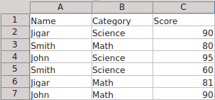
Supposing we have the following data.
We want to create a pivot table of our choice and requirement. So we choose → .
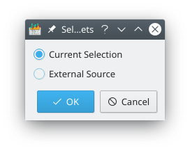
The dialog box that will appear allows user to select the source of data. The data can be taken from the current worksheet or from an external source like a database or ODS file.
Here is the dialog box which allows the user to customize the pivot table. The column labels in the source data are converted to labels which serve as the working fields. The labels can be dragged and dropped into one of three areas (Rows, Columns or Values) to generate the pivot table. You can reset your choices using button.
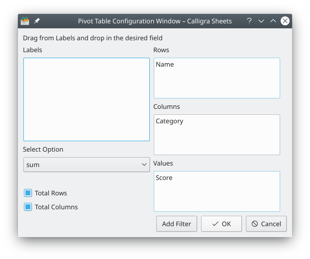
In our example, Name is dragged to Rows, Category to Columns, Score to Values. User defined functions like sum, average, max, min, count, etc. can be selected from the Select Option list.
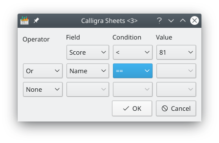
The button can be used to open filter dialog box to filter the desired data. Using this box you can define multiple filters based on the column label and the relationship between them ( or ). This would allow extreme freedom to customize the output.
Total Rows and Total Columns: checking these allow automatic totalling of corresponding rows and columns in the pivot table.